GeezerVison

The World Wide Web, restored to 800 pixels of glory.

GeezerVison is showing ncas-cms.github.io (truncated) — Tutorial — Documentation

Tutorial¶

Version 3.21.0 for version 1.13 of the CF conventions.

All of the Python code in this tutorial is available in two executable scripts (download, 28kB, download, 8kB).

Sample datasets¶

This tutorial uses a number of small sample datasets, all of which can be found in the zip file cf_tutorial_files.zip (download, 164kB):

Unpack the sample datasets.¶

$ unzip -q cf_tutorial_files.zip
$ ls -1
air_temperature.nc
cf_tutorial_files.zip
contiguous.nc
external.nc
file2.nc
file.nc
gathered.nc
parent.nc
precipitation_flux.nc
timeseries.nc
umfile.pp
vertical.nc
wind_components.nc

The tutorial examples assume that the Python session is being run from the directory that contains the zip file and its unpacked contents, and no other files.

The tutorial files may be also found in the downloads directory of the on-line code repository.

It is possible to change the extent to which cf outputs feedback messages and it may be instructive to increase the verbosity whilst working through this tutorial to see and learn more about what cf is doing under the hood and about the nature of the dataset being operated on. See the section on ‘Logging’ for more information.

CF version ¶

The version of the CF conventions and the CF data model being used may be found with the cf.CF function:

Retrieve the version of the CF conventions.¶

>>> cf.CF()
'1.8'

This indicates which version of the CF conventions are represented by this release of the cf package, and therefore the version can not be changed.

Note, however, that datasets of different CF versions may be read from, or written to netCDF.

Field and domain constructs¶

The central constructs of CF are the field construct and domain construct.

The field construct, that corresponds to a CF-netCDF data variable, includes all of the metadata to describe it:

descriptive properties that apply to field construct as a whole (e.g. the standard name),

a data array, and

“metadata constructs” that describe the locations of each cell (i.e. the “domain”) of the data array, and the physical nature of each cell’s datum.

Likewise, the domain construct, that corresponds to a CF-netCDF domain variable or to the domain of a field construct, includes all of the metadata to describe it:

descriptive properties that apply to field construct as a whole (e.g. the long name), and

metadata constructs that describe the locations of each cell of the domain.

A field construct or domain construct is stored in a cf.Field instance or cf.Domain instance respectively. Henceforth the phrase “field construct” will be assumed to mean “cf.Field instance”, and “domain construct” will be assumed to mean “cf.Domain instance”.

Reading field constructs from datasets¶

The cf.read function reads files from disk, or from an OPeNDAP URLs [1], and returns the contents in a cf.FieldList instance that contains zero or more field constructs.

A field list is very much like a Python list, with the addition of extra methods that operate on its field construct elements.

The following file types can be read:

All formats of netCDF3 and netCDF4 files can be read, containing datasets for any version of CF up to and including CF-1.13, including UGRID datasets.

Files in CDL format, with or without the data array values.

Datasets in Zarr v2 (xarray-style) and Zarr v3 formats.

Datasets in Kerchunk format.

PP and UM fields files, whose contents are mapped into field constructs.

Note that when reading netCDF4 files that contain hierachical groups, the group structure is saved via the netCDF interface so that it may be re-used, or modified, if the field constructs are written to back to disk.

For example, to read the file file.nc (found in the sample datasets), which contains two field constructs:

Read file.nc and show that the result is a two-element field list.¶

>>> x = cf.read('file.nc')
>>> type(x)
<class 'cf.fieldlist.FieldList'>
>>> len(x)
2

Descriptive properties are always read into memory, but lazy loading is employed for all data arrays, which means that no data is read into memory until the data is required for inspection or to modify the array contents. This maximises the number of field constructs that may be read within a session, and makes the read operation fast.

Multiple files may be read in one command using UNIX wild card characters, or a sequence of file names (each element of which may also contain wild cards). Shell environment variables are also permitted.

Read the ten sample netCDF files, noting that they contain more than ten field constructs.¶

>>> y = cf.read('*.nc')
>>> len(y)
14

Read two particular files, noting that they contain more than two field constructs.¶

>>> z = cf.read(['file.nc', 'precipitation_flux.nc'])
>>> len(z)
3

All of the datasets in one or more directories may also be read by replacing any file name with a directory name. An attempt will be made to read all files in the directory, which will result in an error if any have a non-supported format. Non-supported files may be ignored by being more specific about the file type intended for reading in using the dataset_type keyword:

Read all of the files in the current working directory.¶

>>> y = cf.read('$PWD')  # Raises Exception
Traceback (most recent call last):
    ...
Exception: Can't determine format of file cf_tutorial_files.zip
>>> y = cf.read('$PWD', dataset_type='netCDF')
>>> len(y)
15

In all cases, the default behaviour is to aggregate the contents of all input datasets into as few field constructs as possible, and it is these aggregated field constructs are returned by cf.read. See the section on aggregation for full details.

The cf.read function has optional parameters to

allow the user to provide files that contain external variables;
request extra field constructs to be created from “metadata” netCDF variables, i.e. those that are referenced from CF-netCDF data variables, but which are not regarded by default as data variables in their own right;
return only domain constructs derived from CF-netCDF domain variables;
request that masking is not applied by convention to data elements (see data masking);
issue warnings when valid_min, valid_max and valid_range attributes are present (see data masking);
display information and issue warnings about the mapping of the netCDF file contents to CF data model constructs;
remove from, or include, size one dimensions on the field constructs’ data;
configure the field construct aggregation process;
configure the reading of directories to allow sub-directories to be read recursively, and to allow directories which resolve to symbolic links; and
choose either netCDF4 or h5netcdf backends for accessing netCDF files.
configure parameters for reading PP and UM fields files.

CF-compliance ¶

If the dataset is partially CF-compliant to the extent that it is not possible to unambiguously map an element of the netCDF dataset to an element of the CF data model, then a field construct is still returned, but may be incomplete. This is so that datasets which are partially conformant may nonetheless be modified in memory and written to new datasets. Such “structural” non-compliance would occur, for example, if the coordinates attribute of a CF-netCDF data variable refers to another variable that does not exist, or refers to a variable that spans a netCDF dimension that does not apply to the data variable. Other types of non-compliance are not checked, such whether or not controlled vocabularies have been adhered to. The structural compliance of the dataset may be checked with the dataset_compliance method of the field construct, as well as optionally displayed when the dataset is read.

Inspection¶

The contents of a field construct may be inspected at three different levels of detail.

Minimal detail ¶

The built-in repr function, invoked on a variable by calling that variable alone at the interpreter prompt, returns a short, one-line description:

Inspect the contents of the two field constructs from the dataset and create a Python variable for each of them.¶

>>> x = cf.read('file.nc')
>>> x
[<CF Field: specific_humidity(latitude(5), longitude(8)) 1>,
 <CF Field: air_temperature(atmosphere_hybrid_height_coordinate(1), grid_latitude(10), grid_longitude(9)) K>]
>>> q = x[0]
>>> t = x[1]
>>> q
<CF Field: specific_humidity(latitude(5), longitude(8)) 1>

This gives the identity of the field construct (e.g. “specific_humidity”), the identities and sizes of the dimensions spanned by the data array (“latitude” and “longitude” with sizes 5 and 8 respectively) and the units of the data (“1”, i.e. dimensionless).

Medium detail ¶

The built-in str function, invoked by a print call on a field construct, returns similar information as the one-line output, along with short descriptions of the metadata constructs, which include the first and last values of their data arrays:

Inspect the contents of the two field constructs with medium detail.¶

>>> print(q)
Field: specific_humidity (ncvar%q)
----------------------------------
Data            : specific_humidity(latitude(5), longitude(8)) 1
Cell methods    : area: mean
Dimension coords: latitude(5) = [-75.0, ..., 75.0] degrees_north
                : longitude(8) = [22.5, ..., 337.5] degrees_east
                : time(1) = [2019-01-01 00:00:00]
>>> print(t)
Field: air_temperature (ncvar%ta)
---------------------------------
Data            : air_temperature(atmosphere_hybrid_height_coordinate(1), grid_latitude(10), grid_longitude(9)) K
Cell methods    : grid_latitude(10): grid_longitude(9): mean where land (interval: 0.1 degrees) time(1): maximum
Field ancils    : air_temperature standard_error(grid_latitude(10), grid_longitude(9)) = [[0.76, ..., 0.32]] K
Dimension coords: atmosphere_hybrid_height_coordinate(1) = [1.5]
                : grid_latitude(10) = [2.2, ..., -1.76] degrees
                : grid_longitude(9) = [-4.7, ..., -1.18] degrees
                : time(1) = [2019-01-01 00:00:00]
Auxiliary coords: latitude(grid_latitude(10), grid_longitude(9)) = [[53.941, ..., 50.225]] degrees_N
                : longitude(grid_longitude(9), grid_latitude(10)) = [[2.004, ..., 8.156]] degrees_E
                : long_name=Grid latitude name(grid_latitude(10)) = [--, ..., b'kappa']
Cell measures   : measure:area(grid_longitude(9), grid_latitude(10)) = [[2391.9657, ..., 2392.6009]] km2
Coord references: grid_mapping_name:rotated_latitude_longitude
                : standard_name:atmosphere_hybrid_height_coordinate
Domain ancils   : ncvar%a(atmosphere_hybrid_height_coordinate(1)) = [10.0] m
                : ncvar%b(atmosphere_hybrid_height_coordinate(1)) = [20.0]
                : surface_altitude(grid_latitude(10), grid_longitude(9)) = [[0.0, ..., 270.0]] m

Note that time values are converted to date-times with the cftime package.

Full detail ¶

The dump method of the field construct gives all properties of all constructs, including metadata constructs and their components, and shows the first and last values of all data arrays:

Inspect the contents of the two field constructs with full detail.¶

>>> q.dump()
----------------------------------
Field: specific_humidity (ncvar%q)
----------------------------------
Conventions = 'CF-1.11'
project = 'research'
standard_name = 'specific_humidity'
units = '1'

Data(latitude(5), longitude(8)) = [[0.003, ..., 0.032]] 1

Cell Method: area: mean

Domain Axis: latitude(5)
Domain Axis: longitude(8)
Domain Axis: time(1)

Dimension coordinate: latitude
    standard_name = 'latitude'
    units = 'degrees_north'
    Data(latitude(5)) = [-75.0, ..., 75.0] degrees_north
    Bounds:Data(latitude(5), 2) = [[-90.0, ..., 90.0]]

Dimension coordinate: longitude
    standard_name = 'longitude'
    units = 'degrees_east'
    Data(longitude(8)) = [22.5, ..., 337.5] degrees_east
    Bounds:Data(longitude(8), 2) = [[0.0, ..., 360.0]]

Dimension coordinate: time
    standard_name = 'time'
    units = 'days since 2018-12-01'
    Data(time(1)) = [2019-01-01 00:00:00]

>>> t.dump()
---------------------------------
Field: air_temperature (ncvar%ta)
---------------------------------
Conventions = 'CF-1.11'
project = 'research'
standard_name = 'air_temperature'
units = 'K'

Data(atmosphere_hybrid_height_coordinate(1), grid_latitude(10), grid_longitude(9)) = [[[0.0, ..., 89.0]]] K

Cell Method: grid_latitude(10): grid_longitude(9): mean where land (interval: 0.1 degrees)
Cell Method: time(1): maximum

Field Ancillary: air_temperature standard_error
    standard_name = 'air_temperature standard_error'
    units = 'K'
    Data(grid_latitude(10), grid_longitude(9)) = [[0.76, ..., 0.32]] K

Domain Axis: atmosphere_hybrid_height_coordinate(1)
Domain Axis: grid_latitude(10)
Domain Axis: grid_longitude(9)
Domain Axis: time(1)

Dimension coordinate: atmosphere_hybrid_height_coordinate
    computed_standard_name = 'altitude'
    standard_name = 'atmosphere_hybrid_height_coordinate'
    Data(atmosphere_hybrid_height_coordinate(1)) = [1.5]
    Bounds:Data(atmosphere_hybrid_height_coordinate(1), 2) = [[1.0, 2.0]]

Dimension coordinate: grid_latitude
    standard_name = 'grid_latitude'
    units = 'degrees'
    Data(grid_latitude(10)) = [2.2, ..., -1.76] degrees
    Bounds:Data(grid_latitude(10), 2) = [[2.42, ..., -1.98]]

Dimension coordinate: grid_longitude
    standard_name = 'grid_longitude'
    units = 'degrees'
    Data(grid_longitude(9)) = [-4.7, ..., -1.18] degrees
    Bounds:Data(grid_longitude(9), 2) = [[-4.92, ..., -0.96]]

Dimension coordinate: time
    standard_name = 'time'
    units = 'days since 2018-12-01'
    Data(time(1)) = [2019-01-01 00:00:00]

Auxiliary coordinate: latitude
    standard_name = 'latitude'
    units = 'degrees_N'
    Data(grid_latitude(10), grid_longitude(9)) = [[53.941, ..., 50.225]] degrees_N

Auxiliary coordinate: longitude
    standard_name = 'longitude'
    units = 'degrees_E'
    Data(grid_longitude(9), grid_latitude(10)) = [[2.004, ..., 8.156]] degrees_E

Auxiliary coordinate: long_name=Grid latitude name
    long_name = 'Grid latitude name'
    Data(grid_latitude(10)) = [--, ..., 'kappa']

Domain ancillary: ncvar%a
    units = 'm'
    Data(atmosphere_hybrid_height_coordinate(1)) = [10.0] m
    Bounds:Data(atmosphere_hybrid_height_coordinate(1), 2) = [[5.0, 15.0]]

Domain ancillary: ncvar%b
    Data(atmosphere_hybrid_height_coordinate(1)) = [20.0]
    Bounds:Data(atmosphere_hybrid_height_coordinate(1), 2) = [[14.0, 26.0]]

Domain ancillary: surface_altitude
    standard_name = 'surface_altitude'
    units = 'm'
    Data(grid_latitude(10), grid_longitude(9)) = [[0.0, ..., 270.0]] m

Coordinate reference: atmosphere_hybrid_height_coordinate
    Coordinate conversion:computed_standard_name = altitude
    Coordinate conversion:standard_name = atmosphere_hybrid_height_coordinate
    Coordinate conversion:a = Domain Ancillary: ncvar%a
    Coordinate conversion:b = Domain Ancillary: ncvar%b
    Coordinate conversion:orog = Domain Ancillary: surface_altitude
    Datum:earth_radius = 6371007
    Dimension Coordinate: atmosphere_hybrid_height_coordinate

Coordinate reference: rotated_latitude_longitude
    Coordinate conversion:grid_mapping_name = rotated_latitude_longitude
    Coordinate conversion:grid_north_pole_latitude = 38.0
    Coordinate conversion:grid_north_pole_longitude = 190.0
    Datum:earth_radius = 6371007
    Dimension Coordinate: grid_longitude
    Dimension Coordinate: grid_latitude
    Auxiliary Coordinate: longitude
    Auxiliary Coordinate: latitude

Cell measure: measure:area
    units = 'km2'
    Data(grid_longitude(9), grid_latitude(10)) = [[2391.9657, ..., 2392.6009]] km2

File inspection with cfa ¶

The description for every field constructs found in datasets also be generated from the command line, with minimal, medium or full detail, by using the cfa tool, for example:

Use cfa on the command line to inspect the field constructs contained in one or more datasets. The “-1” option treats all input files collectively as a single CF dataset, so that aggregation is attempted within and between the input files.¶

$ cfa file.nc
CF Field: air_temperature(atmosphere_hybrid_height_coordinate(1), grid_latitude(10), grid_longitude(9)) K
CF Field: specific_humidity(latitude(5), longitude(8)) 1
$ cfa -1 *.nc
CF Field: specific_humidity(cf_role=timeseries_id(4), ncdim%timeseries(9))
CF Field: cell_area(ncdim%longitude(9), ncdim%latitude(10)) m2
CF Field: eastward_wind(latitude(10), longitude(9)) m s-1
CF Field: specific_humidity(latitude(5), longitude(8)) 1
CF Field: air_potential_temperature(time(120), latitude(5), longitude(8)) K
CF Field: precipitation_flux(time(1), latitude(64), longitude(128)) kg m-2 day-1
CF Field: precipitation_flux(time(2), latitude(4), longitude(5)) kg m2 s-1
CF Field: air_temperature(time(2), latitude(73), longitude(96)) K
CF Field: air_temperature(atmosphere_hybrid_height_coordinate(1), grid_latitude(10), grid_longitude(9)) K

cfa may also be used to write aggregated field constructs to new datasets, and may be used with external files.

Visualisation¶

Powerful, flexible, and user-friendly visualisations of field constructs are available with the 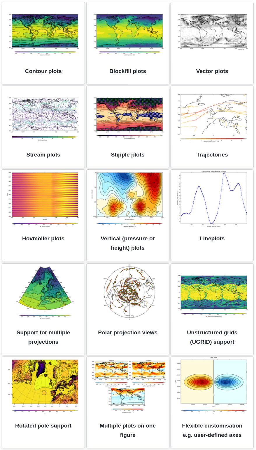cf-plot package (that needs to be installed separately to cf, see cf-plot documentation for details).

_images/new_gallery_view.png — *Examples gallery of plots made with the cf-plot library.*¶

See the cf-plot gallery for the wide range of plotting possibilities, with example code. These include, but are not limited to:

Cylindrical, polar stereographic and other plane projections
Latitude or longitude vs. height or pressure
Hovmuller
Vectors
Stipples
Multiple plots on a page
Colour scales
User defined axes
Rotated pole
Irregular grids
Trajectories
Line plots

Field lists¶

A field list, contained in a cf.FieldList instance, is an ordered sequence of field constructs. It supports all of the Python list operations, such as indexing, iteration, and methods like append.

List-like operations on field list instances.¶

>>> x = cf.read('file.nc')
>>> y = cf.read('precipitation_flux.nc')
>>> x
[<CF Field: specific_humidity(latitude(5), longitude(8)) 1>,
 <CF Field: air_temperature(atmosphere_hybrid_height_coordinate(1), grid_latitude(10), grid_longitude(9)) K>]
>>> y
[<CF Field: precipitation_flux(time(1), latitude(64), longitude(128)) kg m-2 day-1>]
>>> y.extend(x)
>>> y
[<CF Field: precipitation_flux(time(1), latitude(64), longitude(128)) kg m-2 day-1>,
 <CF Field: specific_humidity(latitude(5), longitude(8)) 1>,
 <CF Field: air_temperature(atmosphere_hybrid_height_coordinate(1), grid_latitude(10), grid_longitude(9)) K>]
>>> y[2]
<CF Field: air_temperature(atmosphere_hybrid_height_coordinate(1), grid_latitude(10), grid_longitude(9)) K>
>>> y[::-1]
[<CF Field: air_temperature(atmosphere_hybrid_height_coordinate(1), grid_latitude(10), grid_longitude(9)) K>,
 <CF Field: specific_humidity(latitude(5), longitude(8)) 1>,
 <CF Field: precipitation_flux(time(1), latitude(64), longitude(128)) kg m-2 day-1>]
>>> len(y)
3
>>> len(y + y)
6
>>> len(y * 4)
12
>>> for f in y:
...     print('field:', repr(f))
...
field: <CF Field: precipitation_flux(time(1), latitude(64), longitude(128)) kg m-2 day-1>
field: <CF Field: specific_humidity(latitude(5), longitude(8)) 1>
field: <CF Field: air_temperature(atmosphere_hybrid_height_coordinate(1), grid_latitude(10), grid_longitude(9)) K>

The field list also has some additional methods for copying, testing equality, sorting and selection.

Properties¶

Descriptive properties that apply to field construct as a whole may be retrieved with the properties method:

Retrieve all of the descriptive properties¶

>>> t = cf.read('file.nc')[1]
>>> t.properties()
{'Conventions': 'CF-1.11',
 'project': 'research',
 'standard_name': 'air_temperature',
 'units': 'K'}

Note

From a Python script or using the standard Python shell, the result of methods such as the property methods given here will be returned in condensed form, without linebreaks between items.

If a “pretty printed” output as displayed in these pages is preferred, use the ipython shell or wrap calls with a suitable method from Python’s dedicated pprint module.

Individual properties may be accessed and modified with the del_property, get_property, has_property, and set_property methods:

Check is a property exists, retrieve its value, delete it and then set it to a new value.¶

>>> t.has_property('standard_name')
True
>>> t.get_property('standard_name')
'air_temperature'
>>> t.del_property('standard_name')
'air_temperature'
>>> t.get_property('standard_name', default='not set')
'not set'
>>> t.set_property('standard_name', value='air_temperature')
>>> t.get_property('standard_name', default='not set')
'air_temperature'

A collection of properties may be set at the same time with the set_properties method of the field construct, and all or some properties may be removed with the clear_properties and del_properties methods respectively.

Update the properties with a collection, delete all of the properties, and reinstate the original properties.¶

>>> original = t.properties()
>>> original
{'Conventions': 'CF-1.11',
 'project': 'research',
 'standard_name': 'air_temperature',
 'units': 'K'}
>>> t.set_properties({'foo': 'bar', 'units': 'K'})
>>> t.properties()
{'Conventions': 'CF-1.11',
 'foo': 'bar',
 'project': 'research',
 'standard_name': 'air_temperature',
 'units': 'K'}
>>> t.clear_properties()
 {'Conventions': 'CF-1.11',
 'foo': 'bar',
 'project': 'research',
 'standard_name': 'air_temperature',
 'units': 'K'}
>>> t.properties()
{'units': 'K'}
>>> t.set_properties(original)
>>> t.properties()
{'Conventions': 'CF-1.11',
 'project': 'research',
 'standard_name': 'air_temperature',
 'units': 'K'}

Note that the units property persisted after the call to the clear_properties method because is it deeply associated with the field construct’s data, which still exists.

All of the methods related to the properties are listed here.

Field identities ¶

A field construct identity is a string that describes the construct and is based on the field construct’s properties. A canonical identity is returned by the identity method of the field construct, and all possible identities are returned by the identities method.

A field construct’s identity may be any one of the following

The value of the standard_name property, e.g. 'air_temperature',
The value of the id attribute, preceded by 'id%=',
The value of any property, preceded by the property name and an equals, e.g. 'long_name=Air Temperature', 'foo=bar', etc.,
The netCDF variable name, preceded by “ncvar%”, e.g. 'ncvar%tas' (see the netCDF interface),

Get the canonical identity, and all identities, of a field construct.¶

>>> t.identity()
'air_temperature'
>>> t.identities()
['air_temperature',
 'Conventions=CF-1.11',
 'project=research',
 'units=K',
 'standard_name=air_temperature',
 'ncvar%ta']

The identity returned by the identity method is, by default, the least ambiguous identity (defined in the method documentation), but it may be restricted to the standard_name property and id attribute; or also the long_name property and netCDF variable name (see the netCDF interface). See the strict and relaxed keywords.

Metadata constructs¶

The metadata constructs describe the field construct that contains them. Each CF data model metadata construct has a corresponding cf class:

Class	CF data model construct	Description
`cf.DomainAxis`	Domain axis	Independent axes of the domain
`cf.DimensionCoordinate`	Dimension coordinate	Domain cell locations
`cf.AuxiliaryCoordinate`	Auxiliary coordinate	Domain cell locations
`cf.CoordinateReference`	Coordinate reference	Domain coordinate systems
`cf.DomainAncillary`	Domain ancillary	Cell locations in alternative coordinate systems
`cf.CellMeasure`	Cell measure	Domain cell size or shape
`cf.FieldAncillary`	Field ancillary	Ancillary metadata which vary within the domain
`cf.CellMethod`	Cell method	Describes how data represent variation within cells

Metadata constructs of a particular type can be retrieved with the following attributes of the field construct:

Attribute	Metadata constructs
`domain_axes`	Domain axes
`dimension_coordinates`	Dimension coordinates
`auxiliary_coordinates`	Auxiliary coordinates
`coordinate_references`	Coordinate references
`domain_ancillaries`	Domain ancillaries
`cell_measures`	Cell measures
`field_ancillaries`	Field ancillaries
`cell_methods`	Cell methods

Each of these attributes returns a cf.Constructs class instance that maps metadata constructs to unique identifiers called “construct keys”. A cf.Constructs instance has methods for selecting constructs that meet particular criteria (see Filtering metadata constructs). It also behaves like a “read-only” Python dictionary, in that it has items, keys and values methods that work exactly like their corresponding dict methods. It also has a get method and indexing like a Python dictionary (see Metadata construct access for details).

Retrieve the field construct’s coordinate reference constructs, and access them using dictionary methods.¶

>>> q, t = cf.read('file.nc')
>>> t.coordinate_references
<CF Constructs: coordinate_reference(2)>
>>> print(t.coordinate_references)
Constructs:
{'coordinatereference0': <CF CoordinateReference: standard_name:atmosphere_hybrid_height_coordinate>,
 'coordinatereference1': <CF CoordinateReference: grid_mapping_name:rotated_latitude_longitude>}
>>> list(t.coordinate_references().keys())
['coordinatereference0', 'coordinatereference1']
>>> for key, value in t.coordinate_references().items():
...     print(key, repr(value))
...
coordinatereference0 <CF CoordinateReference: standard_name:atmosphere_hybrid_height_coordinate>
coordinatereference1 <CF CoordinateReference: grid_mapping_name:rotated_latitude_longitude>

Retrieve the field construct’s dimension coordinate and domain axis constructs.¶

>>> print(t.dimension_coordinates)
Constructs:
{'dimensioncoordinate0': <CF DimensionCoordinate: atmosphere_hybrid_height_coordinate(1) >,
 'dimensioncoordinate1': <CF DimensionCoordinate: grid_latitude(10) degrees>,
 'dimensioncoordinate2': <CF DimensionCoordinate: grid_longitude(9) degrees>,
 'dimensioncoordinate3': <CF DimensionCoordinate: time(1) days since 2018-12-01 >}
>>> print(t.domain_axes)
Constructs:
{'domainaxis0': <CF DomainAxis: size(1)>,
 'domainaxis1': <CF DomainAxis: size(10)>,
 'domainaxis2': <CF DomainAxis: size(9)>,
 'domainaxis3': <CF DomainAxis: size(1)>}

The construct keys (e.g. 'domainaxis1') are usually generated internally and are unique within the field construct. However, construct keys may be different for equivalent metadata constructs from different field constructs, and for different Python sessions.

Metadata constructs of all types may be returned by the constructs attribute of the field construct:

Retrieve all of the field construct’s metadata constructs.¶

>>> q.constructs
<CF Constructs: cell_method(1), dimension_coordinate(3), domain_axis(3)>
>>> print(q.constructs)
Constructs:
{'cellmethod0': <CF CellMethod: area: mean>,
 'dimensioncoordinate0': <CF DimensionCoordinate: latitude(5) degrees_north>,
 'dimensioncoordinate1': <CF DimensionCoordinate: longitude(8) degrees_east>,
 'dimensioncoordinate2': <CF DimensionCoordinate: time(1) days since 2018-12-01 >,
 'domainaxis0': <CF DomainAxis: size(5)>,
 'domainaxis1': <CF DomainAxis: size(8)>,
 'domainaxis2': <CF DomainAxis: size(1)>}
>>> t.constructs
<CF Constructs: auxiliary_coordinate(3), cell_measure(1), cell_method(2), coordinate_reference(2), dimension_coordinate(4), domain_ancillary(3), domain_axis(4), field_ancillary(1)>
>>> print(t.constructs)
Constructs:
{'auxiliarycoordinate0': <CF AuxiliaryCoordinate: latitude(10, 9) degrees_N>,
 'auxiliarycoordinate1': <CF AuxiliaryCoordinate: longitude(9, 10) degrees_E>,
 'auxiliarycoordinate2': <CF AuxiliaryCoordinate: long_name=Grid latitude name(10) >,
 'cellmeasure0': <CF CellMeasure: measure:area(9, 10) km2>,
 'cellmethod0': <CF CellMethod: domainaxis1: domainaxis2: mean where land (interval: 0.1 degrees)>,
 'cellmethod1': <CF CellMethod: domainaxis3: maximum>,
 'coordinatereference0': <CF CoordinateReference: standard_name:atmosphere_hybrid_height_coordinate>,
 'coordinatereference1': <CF CoordinateReference: grid_mapping_name:rotated_latitude_longitude>,
 'dimensioncoordinate0': <CF DimensionCoordinate: atmosphere_hybrid_height_coordinate(1) >,
 'dimensioncoordinate1': <CF DimensionCoordinate: grid_latitude(10) degrees>,
 'dimensioncoordinate2': <CF DimensionCoordinate: grid_longitude(9) degrees>,
 'dimensioncoordinate3': <CF DimensionCoordinate: time(1) days since 2018-12-01 >,
 'domainancillary0': <CF DomainAncillary: ncvar%a(1) m>,
 'domainancillary1': <CF DomainAncillary: ncvar%b(1) >,
 'domainancillary2': <CF DomainAncillary: surface_altitude(10, 9) m>,
 'domainaxis0': <CF DomainAxis: size(1)>,
 'domainaxis1': <CF DomainAxis: size(10)>,
 'domainaxis2': <CF DomainAxis: size(9)>,
 'domainaxis3': <CF DomainAxis: size(1)>,
 'fieldancillary0': <CF FieldAncillary: air_temperature standard_error(10, 9) K>}

Data¶

The field construct’s data is stored in a cf.Data class instance that is accessed with the data attribute of the field construct.

Retrieve the data and inspect it, showing the shape and some illustrative values.¶

>>> q, t = cf.read('file.nc')
>>> t.data
<CF Data(1, 10, 9): [[[262.8, ..., 269.7]]] K>

The cf.Data instance provides access to the full array of values, as well as attributes to describe the array and methods for describing any data compression. The field construct also has a get_data method as an alternative means of retrieving the data instance, which allows for a default to be returned if no data have been set; as well as a del_data method for removing the data.

The field construct (and any other construct that contains data) also provides attributes for direct access.

Retrieve a numpy array of the data.¶

>>> a = t.array
>>> type(a)
numpy.ma.core.MaskedArray
>>> print(a)
[[[262.8 270.5 279.8 269.5 260.9 265.0 263.5 278.9 269.2]
  [272.7 268.4 279.5 278.9 263.8 263.3 274.2 265.7 279.5]
  [269.7 279.1 273.4 274.2 279.6 270.2 280.  272.5 263.7]
  [261.7 260.6 270.8 260.3 265.6 279.4 276.9 267.6 260.6]
  [264.2 275.9 262.5 264.9 264.7 270.2 270.4 268.6 275.3]
  [263.9 263.8 272.1 263.7 272.2 264.2 260.  263.5 270.2]
  [273.8 273.1 268.5 272.3 264.3 278.7 270.6 273.0 270.6]
  [267.9 273.5 279.8 260.3 261.2 275.3 271.2 260.8 268.9]
  [270.9 278.7 273.2 261.7 271.6 265.8 273.  278.5 266.4]
  [276.4 264.2 276.3 266.1 276.1 268.1 277.  273.4 269.7]]]

Inspect the data type, number of dimensions, dimension sizes and number of elements of the data.¶

>>> t.dtype
dtype('float64')
>>> t.ndim
3
>>> t.shape
(1, 10, 9)
>>> t.size
90

The array is stored internally as a Dask array, which can be retrieved with the to_dask_array() method of the field construct:

Retrieve the dask array of the data.¶

>>> d = t.to_dask_array()
>>> d
dask.array<array, shape=(1, 10, 9), dtype=float64, chunksize=(1, 10, 9), chunktype=numpy.ndarray>

Note that changes to the returned Dask array in-place will also be seen in the field construct.

All of the methods and attributes related to the data are listed here.

Data axes ¶

The data array of the field construct spans all the domain axis constructs with the possible exception of size one domain axis constructs. The domain axis constructs spanned by the field construct’s data are found with the get_data_axes method of the field construct. For example, the data of the field construct t does not span the size one domain axis construct with key 'domainaxis3'.

Show which data axis constructs are spanned by the field construct’s data.¶

>>> print(t.domain_axes)
Constructs:
{'domainaxis0': <CF DomainAxis: size(1)>,
 'domainaxis1': <CF DomainAxis: size(10)>,
 'domainaxis2': <CF DomainAxis: size(9)>,
 'domainaxis3': <CF DomainAxis: size(1)>}
>>> t
<CF Field: air_temperature(atmosphere_hybrid_height_coordinate(1), grid_latitude(10), grid_longitude(9)) K>
>>> t.data.shape
(1, 10, 9)
>>> t.get_data_axes()
('domainaxis0', 'domainaxis1', 'domainaxis2')

The data may be set with the set_data method of the field construct. The domain axis constructs spanned by the data are inferred from the existing domain axis constructs, provided that there are no ambiguities (such as two dimensions of the same size), in which case they can be explicitly provided via their construct keys. In any case, the data axes may be set at any time with the set_data_axes method of the field construct.

Delete the data and then reinstate it, using the existing data axes.¶

>>> data = t.del_data()
>>> t.has_data()
False
>>> t.set_data(data)
>>> t.data
<CF Data(1, 10, 9): [[[262.8, ..., 269.7]]] K>

See the section field construct creation for more examples.

Date-time ¶

Data representing date-times is defined as elapsed times since a reference date-time in a particular calendar (Gregorian, by default). The array attribute of the cf.Data instance (and any construct that contains it) returns the elapsed times, and the datetime_array (and any construct that contains it) returns the data as an array of date-time objects.

View date-times as elapsed time or as date-time objects.¶

>>> d = cf.Data([1, 2, 3], units='days since 2004-2-28')
>>> print(d.array)
[1 2 3]
>>> print(d.datetime_array)
[cftime.DatetimeGregorian(2004-02-29 00:00:00)
 cftime.DatetimeGregorian(2004-03-01 00:00:00)
 cftime.DatetimeGregorian(2004-03-02 00:00:00)]
>>> e = cf.Data([1, 2, 3], units='days since 2004-2-28', calendar='360_day')
>>> print(e.array)
[1 2 3]
>>> print(e.datetime_array)
[cftime.Datetime360Day(2004-02-29 00:00:00)
 cftime.Datetime360Day(2004-02-30 00:00:00)
 cftime.Datetime360Day(2004-03-01 00:00:00)]

Alternatively, date-time data may be created by providing date-time objects or ISO 8601-like date-time strings. Date-time objects may be cftime.datetime instances (as returned by the cf.dt and cf.dt_vector functions), Python datetime.datetime instances, or any other date-time object that has an equivalent API.

Creating a Data instance from a date-time objects.¶

>>> date_time = cf.dt(2004, 2, 29)
>>> date_time
cftime.datetime(2004-02-29 00:00:00)
>>> d = cf.Data(date_time, calendar='gregorian')
>>> print(d.array)
0.0
>>> d.datetime_array
array(cftime.DatetimeGregorian(2004-02-29 00:00:00), dtype=object)

Creating Data instances from date-time an array of date-time objects.¶

>>> date_times  = cf.dt_vector(['2004-02-29', '2004-02-30', '2004-03-01'], calendar='360_day')
>>> print (date_times)
[cftime.Datetime360Day(2004-02-29 00:00:00)
 cftime.Datetime360Day(2004-02-30 00:00:00)
 cftime.Datetime360Day(2004-03-01 00:00:00)]
>>> e = cf.Data(date_times)
>>> print(e.array)
[0. 1. 2.]
>>> print(e.datetime_array)
[cftime.Datetime360Day(2004-02-29 00:00:00)
 cftime.Datetime360Day(2004-02-30 00:00:00)
 cftime.Datetime360Day(2004-03-01 00:00:00)]

Creating Data instances from date-time strings. If no units or calendar are provided then the “dt” keyword is required.¶

>>> d = cf.Data(['2004-02-29', '2004-02-30', '2004-03-01'], calendar='360_day')
>>> d.Units
<Units: days since 2004-02-29 360_day>
>>> print(d.array)
[0. 1. 2.]
>>> print(d.datetime_array)
[cftime.Datetime360Day(2004-02-29 00:00:00)
 cftime.Datetime360Day(2004-02-30 00:00:00)
 cftime.Datetime360Day(2004-03-01 00:00:00)]
>>> e = cf.Data(['2004-02-29', '2004-03-01', '2004-03-02'], dt=True)
>>> e.Units
<Units: days since 2004-02-29>
>>> print(e.datetime_array)
[cftime.DatetimeGregorian(2004-02-29 00:00:00)
 cftime.DatetimeGregorian(2004-03-01 00:00:00)
 cftime.DatetimeGregorian(2004-03-02 00:00:00)]
>>> f = cf.Data(['2004-02-29', '2004-03-01', '2004-03-02'])
>>> print(f.array)
['2004-02-29' '2004-03-01' '2004-03-02']
>>> f.Units
<Units: >
>>> print(f.datetime_array)  # Raises Exception
Traceback (most recent call last):
    ...
ValueError: Can't create date-time array from units <Units: >

Manipulating dimensions ¶

The dimensions of a field construct’s data may be reordered, have size one dimensions removed and have new size one dimensions included by using the following field construct methods:

Method	Description
`flatten`	Flatten domain axes of the field construct
`flip`	Reverse the direction of a data dimension
`insert_dimension`	Insert a new size one data dimension. The new dimension must correspond to an existing size one domain axis construct.
`squeeze`	Remove size one data dimensions
`transpose`	Reorder data dimensions
`unsqueeze`	Insert all missing size one data dimensions

Remove all size one dimensions from the data, noting that metadata constructs which span the corresponding domain axis construct are not affected.¶

>>> q, t = cf.read('file.nc')
>>> t
<CF Field: air_temperature(atmosphere_hybrid_height_coordinate(1), grid_latitude(10), grid_longitude(9)) K>
>>> t2 = t.squeeze()
>>> t2
<CF Field: air_temperature(grid_latitude(10), grid_longitude(9)) K>
>>> print(t2.dimension_coordinates)
Constructs:
{'dimensioncoordinate0': <CF DimensionCoordinate: atmosphere_hybrid_height_coordinate(1) >,
 'dimensioncoordinate1': <CF DimensionCoordinate: grid_latitude(10) degrees>,
 'dimensioncoordinate2': <CF DimensionCoordinate: grid_longitude(9) degrees>,
 'dimensioncoordinate3': <CF DimensionCoordinate: time(1) days since 2018-12-01 >}

Insert a new size one dimension, corresponding to a size one domain axis construct, and then reorder the dimensions.¶

>>> t3 = t2.insert_dimension(axis='domainaxis3', position=1)
>>> t3
<CF Field: air_temperature(grid_latitude(10), time(1), grid_longitude(9)) K>
>>> t3.transpose([2, 0, 1])
<CF Field: air_temperature(grid_longitude(9), grid_latitude(10), time(1)) K>

When transposing the data dimensions, the dimensions of metadata construct data are, by default, unchanged. It is also possible to permute the data dimensions of the metadata constructs so that they have the same relative order as the field construct:

Also permute the data dimension of metadata constructs using the ‘constructs’ keyword.¶

>>> t4 = t.transpose(['X', 'Z', 'Y'], constructs=True)

Data mask ¶

See also

Assignment by condition

There is always a data mask, which may be thought of as a separate data array of Booleans with the same shape as the original data. The data mask is False where the data has values, and True where the data is missing. The data mask may be inspected with the mask attribute of the field construct, which returns the data mask in a field construct with the same metadata constructs as the original field construct.

Inspect the data mask of a field construct.¶

>>> print(q)
Field: specific_humidity (ncvar%q)
----------------------------------
Data            : specific_humidity(latitude(5), longitude(8)) 1
Cell methods    : area: mean
Dimension coords: latitude(5) = [-75.0, ..., 75.0] degrees_north
                : longitude(8) = [22.5, ..., 337.5] degrees_east
                : time(1) = [2019-01-01 00:00:00]
>>> print(q.mask)
Field: long_name=mask
---------------------
Data            : long_name=mask(latitude(5), longitude(8))
Cell methods    : area: mean
Dimension coords: latitude(5) = [-75.0, ..., 75.0] degrees_north
                : longitude(8) = [22.5, ..., 337.5] degrees_east
                : time(1) = [2019-01-01 00:00:00]
>>> print(q.mask.array)
[[False False False False False False False False]
 [False False False False False False False False]
 [False False False False False False False False]
 [False False False False False False False False]
 [False False False False False False False False]]

Mask the polar rows (see the “Assignment by index” section) and inspect the new data mask.¶

>>> q[[0, 4], :] = cf.masked
>>> print(q.mask.array)
[[ True  True  True  True  True  True  True  True]
 [False False False False False False False False]
 [False False False False False False False False]
 [False False False False False False False False]
 [ True  True  True  True  True  True  True  True]]

The _FillValue and missing_value attributes of the field construct are not stored as values of the field construct’s data. They are only used when writing the data to a netCDF dataset. Therefore testing for missing data by testing for equality to one of these property values will produce incorrect results; the any and all methods of the field construct should be used instead.

See if all, or any, data points are masked.¶

>>> q.mask.all()
False
>>> q.mask.any()
True

The mask of a netCDF dataset array is implied by array values that meet the criteria implied by the missing_value, _FillValue, valid_min, valid_max, and valid_range properties, and is usually applied automatically by cf.read. NetCDF data elements that equal the values of the missing_value and _FillValue properties are masked, as are data elements that exceed the value of the valid_max property, succeed the value of the valid_min property, or lie outside of the range defined by the valid_range property.

However, this automatic masking may be bypassed by setting the mask keyword of the cf.read function to False. The mask, as defined in the dataset, may subsequently be applied manually with the apply_masking method of the field construct.

Read a dataset from disk without automatic masking, and then manually apply the mask¶

>>> cf.write(q, 'masked_q.nc')
>>> no_mask_q = cf.read('masked_q.nc', mask=False)[0]
>>> print(no_mask_q.array)
[9.96920997e+36, 9.96920997e+36, 9.96920997e+36, 9.96920997e+36,
 9.96920997e+36, 9.96920997e+36, 9.96920997e+36, 9.96920997e+36],
 [0.023 0.036 0.045 0.062 0.046 0.073 0.006 0.066]
 [0.11  0.131 0.124 0.146 0.087 0.103 0.057 0.011]
 [0.029 0.059 0.039 0.07  0.058 0.072 0.009 0.017]
[9.96920997e+36, 9.96920997e+36, 9.96920997e+36, 9.96920997e+36,
 9.96920997e+36, 9.96920997e+36, 9.96920997e+36, 9.96920997e+36]])
>>> masked_q = no_mask_q.apply_masking()
>>> print(masked_q.array)
[[   --    --    --    --    --    --    --    --]
 [0.023 0.036 0.045 0.062 0.046 0.073 0.006 0.066]
 [0.11  0.131 0.124 0.146 0.087 0.103 0.057 0.011]
 [0.029 0.059 0.039 0.07  0.058 0.072 0.009 0.017]
 [   --    --    --    --    --    --    --    --]]

The apply_masking method of the field construct utilises as many of the missing_value, _FillValue, valid_min, valid_max, and valid_range properties as are present and may be used on any construct, not only those that have been read from datasets.

Subspacing by index¶

Creation of a new field construct which spans a subspace of the domain of an existing field construct is achieved either by indexing the field construct directly (as described in this section) or by identifying indices based on the metadata constructs (see Subspacing by metadata). The subspacing operation, in either case, also subspaces any metadata constructs of the field construct (e.g. coordinate metadata constructs) which span any of the domain axis constructs that are affected. The new field construct is created with the same properties as the original field construct.

Subspacing by indexing uses rules that are very similar to the numpy indexing rules, the only differences being:

An integer index i specified for a dimension reduces the size of this dimension to unity, taking only the i-th element, but keeps the dimension itself, so that the rank of the array is not reduced.

When two or more dimensions’ indices are sequences of integers then these indices work independently along each dimension (similar to the way vector subscripts work in FORTRAN). This is the same indexing behaviour as on a Variable object of the netCDF4 package.

For a dimension that is cyclic, a range of indices specified by a slice that spans the edges of the data (such as -2:3 or 3:-2:-1) is assumed to “wrap” around, rather then producing a null result.

Create a new field construct whose domain spans the first longitude of the original, and with a reversed latitude axis.¶

>>> q, t = cf.read('file.nc')
>>> print(q)
Field: specific_humidity (ncvar%q)
----------------------------------
Data            : specific_humidity(latitude(5), longitude(8)) 1
Cell methods    : area: mean
Dimension coords: time(1) = [2019-01-01 00:00:00]
                : latitude(5) = [-75.0, ..., 75.0] degrees_north
                : longitude(8) = [22.5, ..., 337.5] degrees_east

>>> new = q[::-1, 0]
>>> print(new)
Field: specific_humidity (ncvar%q)
----------------------------------
Data            : specific_humidity(latitude(5), longitude(1)) 1
Cell methods    : area: mean
Dimension coords: time(1) = [2019-01-01 00:00:00]
                : latitude(5) = [75.0, ..., -75.0] degrees_north
                : longitude(1) = [22.5] degrees_east

Create new field constructs with a variety of indexing techniques.¶

>>> t
<CF Field: air_temperature(atmosphere_hybrid_height_coordinate(1), grid_latitude(10), grid_longitude(9)) K>
>>> t[:, :, 1]
<CF Field: air_temperature(atmosphere_hybrid_height_coordinate(1), grid_latitude(10), grid_longitude(1)) K>
>>> t[:, 0]
<CF Field: air_temperature(atmosphere_hybrid_height_coordinate(1), grid_latitude(1), grid_longitude(9)) K>
>>> t[..., 6:3:-1, 3:6]
<CF Field: air_temperature(atmosphere_hybrid_height_coordinate(1), grid_latitude(3), grid_longitude(3)) K>
>>> t[0, [2, 3, 9], [4, 8]]
<CF Field: air_temperature(atmosphere_hybrid_height_coordinate(1), grid_latitude(3), grid_longitude(2)) K>
>>> t[0, :, -2]
<CF Field: air_temperature(atmosphere_hybrid_height_coordinate(1), grid_latitude(10), grid_longitude(1)) K>
>>> t[..., [True, False, True, True, False, False, True, False, False]]
<CF Field: air_temperature(atmosphere_hybrid_height_coordinate(1), grid_latitude(10), grid_longitude(4)) K>

Subspacing a cyclic dimension with a slice will wrap around the data edges.¶

>>> q
<CF Field: specific_humidity(latitude(5), longitude(8)) 1>
>>> q.cyclic()
{'domainaxis1'}
>>> q.constructs.domain_axis_identity('domainaxis1')
'longitude'
>>> print(q[:, -2:3])
Field: specific_humidity (ncvar%q)
----------------------------------
Data            : specific_humidity(latitude(5), longitude(5)) 1
Cell methods    : area: mean
Dimension coords: latitude(5) = [-75.0, ..., 75.0] degrees_north
                : longitude(5) = [-67.5, ..., 112.5] degrees_east
                : time(1) = [2019-01-01 00:00:00]
>>> print(q[:, 3:-2:-1])
Field: specific_humidity (ncvar%q)
----------------------------------
Data            : specific_humidity(latitude(5), longitude(5)) 1
Cell methods    : area: mean
Dimension coords: latitude(5) = [-75.0, ..., 75.0] degrees_north
                : longitude(5) = [157.5, ..., -22.5] degrees_east
                : time(1) = [2019-01-01 00:00:00]

An index that is a list of integers may also be provided as a numpy array, a dask array, a cf.Data instance, or a metadata construct that has data:

Create a new field construct for longitudes greater than 180 degrees east.¶

>>> lon = q.dimension_coordinate('X')
>>> print(q[:, lon > 180])
Field: specific_humidity (ncvar%q)
----------------------------------
Data            : specific_humidity(latitude(5), longitude(4)) 1
Cell methods    : area: mean
Dimension coords: latitude(5) = [-75.0, ..., 75.0] degrees_north
                : longitude(4) = [202.5, ..., 337.5] degrees_east
                : time(1) = [2019-01-01 00:00:00]

A cf.Data instance can also directly be indexed in the same ways:

Create a new ‘Data’ instance by indexing.¶

>>> t.data[0, [2, 3, 9], [4, 8]]
<CF Data(1, 3, 2): [[[279.6, ..., 269.7]]] K>

Assignment by index¶

Data elements can be changed by assigning to elements selected by indices of the data (as described in this section); by conditions based on the data values of the field construct or one of its metadata constructs (see Assignment by condition); or by identifying indices based on arbitrary metadata constructs (see Assignment by metadata).

Assignment by indices uses rules that are very similar to the numpy indexing rules, the only difference being:

When two or more dimensions’ indices are sequences of integers then these indices work independently along each dimension (similar to the way vector subscripts work in FORTRAN). This is the same indexing behaviour as on a Variable object of the netCDF4 package.

For a dimension that is cyclic, a range of indices specified by a slice that spans the edges of the data (such as -2:3 or 3:-2:-1) is assumed to “wrap” around, rather then producing a null result.

A single value may be assigned to any number of elements.

Set a single element to -1, a “column” of elements to -2 and a “square” of elements to -3.¶

>>> q, t = cf.read('file.nc')
>>> t[:, 0, 0] = -1
>>> t[:, :, 1] = -2
>>> t[..., 6:3:-1, 3:6] = -3
>>> print(t.array)
[[[ -1.0  -2.0 279.8 269.5 260.9 265.0 263.5 278.9 269.2]
  [272.7  -2.0 279.5 278.9 263.8 263.3 274.2 265.7 279.5]
  [269.7  -2.0 273.4 274.2 279.6 270.2 280.0 272.5 263.7]
  [261.7  -2.0 270.8 260.3 265.6 279.4 276.9 267.6 260.6]
  [264.2  -2.0 262.5  -3.0  -3.0  -3.0 270.4 268.6 275.3]
  [263.9  -2.0 272.1  -3.0  -3.0  -3.0 260.0 263.5 270.2]
  [273.8  -2.0 268.5  -3.0  -3.0  -3.0 270.6 273.0 270.6]
  [267.9  -2.0 279.8 260.3 261.2 275.3 271.2 260.8 268.9]
  [270.9  -2.0 273.2 261.7 271.6 265.8 273.0 278.5 266.4]
  [276.4  -2.0 276.3 266.1 276.1 268.1 277.0 273.4 269.7]]]

An array of values can be assigned, as long as it is broadcastable to the shape defined by the indices, using the numpy broadcasting rules.

Assigning arrays of values.¶

>>> import numpy
>>> t[..., 6:3:-1, 3:6] = numpy.arange(9).reshape(3, 3)
>>> t[0, [2, 9], [4, 8]] =  cf.Data([[-4, -5]])
>>> t[0, [4, 7], 0] = [[-10], [-11]]
>>> print(t.array)
[[[ -1.0  -2.0 279.8 269.5 260.9 265.0 263.5 278.9 269.2]
  [272.7  -2.0 279.5 278.9 263.8 263.3 274.2 265.7 279.5]
  [269.7  -2.0 273.4 274.2  -4.0 270.2 280.0 272.5  -5.0]
  [261.7  -2.0 270.8 260.3 265.6 279.4 276.9 267.6 260.6]
  [-10.0  -2.0 262.5   6.0   7.0   8.0 270.4 268.6 275.3]
  [263.9  -2.0 272.1   3.0   4.0   5.0 260.0 263.5 270.2]
  [273.8  -2.0 268.5   0.0   1.0   2.0 270.6 273.0 270.6]
  [-11.0  -2.0 279.8 260.3 261.2 275.3 271.2 260.8 268.9]
  [270.9  -2.0 273.2 261.7 271.6 265.8 273.0 278.5 266.4]
  [276.4  -2.0 276.3 266.1  -4.0 268.1 277.0 273.4  -5.0]]]

In-place modification is also possible:

Modifying the data in-place.¶

>>> print(t[0, 0, -1].array)
[[[269.2]]]
>>> t[0, 0, -1] /= -10
>>> print(t[0, 0, -1].array)
[[[-26.92]]]

A cf.Data instance can also assigned values in the same way:

Assign to the ‘Data’ instance directly.¶

>>> t.data[0, 0, -1] = -99
>>> print(t[0, 0, -1].array)
[[[-99.]]]

An index that is a list of integers may also be provided as a numpy array, a dask array, a cf.Data instance, or a metadata construct that has data:

Assign to elements which correspond to positive grid latitudes.¶

>>> y = t.dimension_coordinate('Y')
>>> t[:, y > 0] = -6
>>> print(t)
[[[ -6.0 -4.0  -6.0  -6.0  -6.0  -6.0  -6.0  -6.0  -6.0]
  [ -6.0 -4.0  -6.0  -6.0  -6.0  -6.0  -6.0  -6.0  -6.0]
  [ -6.0 -4.0  -6.0  -6.0  -6.0  -6.0  -6.0  -6.0  -6.0]
  [ -6.0 -4.0  -6.0  -6.0  -6.0  -6.0  -6.0  -6.0  -6.0]
  [ -6.0 -4.0  -6.0  -6.0  -6.0  -6.0  -6.0  -6.0  -6.0]
  [263.9 -2.0 272.1   3.0   4.0   5.0 260.0 263.5 270.2]
  [273.8 -2.0 268.5   0.0   1.0   2.0 270.6 273.0 270.6]
  [-11.0 -2.0 279.8 260.3 261.2 275.3 271.2 260.8 268.9]
  [270.9 -2.0 273.2 261.7 271.6 265.8 273.0 278.5 266.4]
  [276.4 -2.0 276.3 266.1  -4.0 268.1 277.0 273.4  -5.0]]]

Masked values ¶

Data array elements may be set to masked values by assigning them to the cf.masked constant, thereby updating the data mask.

Set a column of elements to masked values.¶

>>> t[0, :, -2] = cf.masked
>>> print(t.array)
[[[ -1.0  -2.0 279.8 269.5 260.9 265.0 263.5    -- -99.0]
  [272.7  -2.0 279.5 278.9 263.8 263.3 274.2    -- 279.5]
  [269.7  -2.0 273.4 274.2  -4.0 270.2 280.0    --  -5.0]
  [261.7  -2.0 270.8 260.3 265.6 279.4 276.9    -- 260.6]
  [264.2  -2.0 262.5   6.0   7.0   8.0 270.4    -- 275.3]
  [263.9  -2.0 272.1   3.0   4.0   5.0 260.0    -- 270.2]
  [273.8  -2.0 268.5   0.0   1.0   2.0 270.6    -- 270.6]
  [-11.0  -2.0 279.8 260.3 261.2 275.3 271.2    -- 268.9]
  [270.9  -2.0 273.2 261.7 271.6 265.8 273.0    -- 266.4]
  [276.4  -2.0 276.3 266.1  -4.0 268.1 277.0    --  -5.0]]]

By default the data mask is “hard”, meaning that masked values can not be changed by assigning them to another value. This behaviour may be changed by setting the hardmask attribute of the field construct to False, thereby making the data mask “soft”.

Changing masked elements back to data values is only possible when the “hardmask” attribute is False.¶

>>> t[0, 4, -2] = 99
>>> print(t[0, 4, -2].array)
[[[--]]]
>>> t.hardmask = False
>>> t[0, 4, -2] = 99
>>> print(t[0, 4, -2].array)
[[[99.]]]

Note that this is the opposite behaviour to numpy arrays, which assume that the mask is soft by default. The reason for the difference is so that land-sea masks are, by default, preserved through assignment operations.

Assignment from other field constructs ¶

Another field construct can also be assigned to indices. The other field construct’s data is actually assigned, but only after being transformed so that it is broadcastable to the subspace defined by the assignment indices. This is done by using the metadata constructs of the two field constructs to create a mapping of physically compatible dimensions between the fields, and then manipulating the dimensions of the other field construct’s data to ensure that they are broadcastable.

Transform a field construct’s data and assign it back to the original field, demonstrating that this is a null operation.¶

>>> q, t = cf.read('file.nc')
>>> t0 = t.copy()
>>> u = t.squeeze(0)
>>> u.transpose(inplace=True)
>>> u.flip(inplace=True)
>>> t[...] = u
>>> t.allclose(t0)
True

Broadcasting is carried out after transforms to ensure field construct compatibility.¶

>>> print(t[:, :, 1:3].array)
[[[270.5 279.8]
   [268.4 279.5]
   [279.1 273.4]
   [260.6 270.8]
   [275.9 262.5]
   [263.8 272.1]
   [273.1 268.5]
   [273.5 279.8]
   [278.7 273.2]
   [264.2 276.3]]]
>>> print(u[2].array)
[[277.  273.  271.2 270.6 260.  270.4 276.9 280.  274.2 263.5]]
>>> t[:, :, 1:3] = u[2]
>>> print(t[:, :, 1:3].array)
[[[263.5 263.5]
  [274.2 274.2]
  [280.  280. ]
  [276.9 276.9]
  [270.4 270.4]
  [260.  260. ]
  [270.6 270.6]
  [271.2 271.2]
  [273.  273. ]
  [277.  277. ]]]

If either of the field constructs does not have sufficient metadata to create the such a mapping, then any manipulation of the dimensions must be done manually, and the other field construct’s cf.Data instance (rather than the field construct itself) may be assigned.

Assignment of bounds ¶

When assigning an object that has bounds to an object that also has bounds, then the bounds are also assigned. This is the only circumstance that allows bounds to be updated during assignment by index.

Units¶

The field construct, and any metadata construct that contains data, has units which are described by the Units attribute that stores a cf.Units object (which is identical to a cfunits.Units object of the cfunits package). The units property provides the units contained in the cf.Units instance, and changes in one are reflected in the other.

Inspection and changing of units.¶

>>> q, t = cf.read('file.nc')
>>> t.units
'K'
>>> t.Units
<Units: K>
>>> t.units = 'degreesC'
>>> t.units
'degreesC'
>>> t.Units
<Units: degreesC>
>>> t.Units += 273.15
>>> t.units
'K'
>>> t.Units
<Units: K>

When the units are changed, the data are automatically converted to the new units when next accessed.

Changing the units automatically results in conversion of the data values.¶

>>> t.data
<CF Data(1, 10, 9): [[[262.8, ..., 269.7]]] K>
>>> t.Units = cf.Units('degreesC')
>>> t.data
<CF Data(1, 10, 9): [[[-10.35, ..., -3.45]]] degreesC>
>>> t.units = 'Kelvin'
>>> t.data
<CF Data(1, 10, 9): [[[262.8, ..., 269.7]]] Kelvin>

When assigning to the data with values that have units, the values are automatically converted to have the same units as the data.

Automatic conversions occur when assigning from data with different units.¶

>>> t.data
<CF Data(1, 10, 9): [[[262.8, ..., 269.7]]] Kelvin>
>>> t[0, 0, 0] = cf.Data(1)
>>> t.data
<CF Data(1, 10, 9): [[[1.0, ..., 269.7]]] Kelvin>
>>> t[0, 0, 0] = cf.Data(1, 'degreesC')
>>> t.data
<CF Data(1, 10, 9): [[[274.15, ..., 269.7]]] Kelvin>

Automatic units conversions are also carried out between operands during mathematical operations.

Calendar ¶

When the data represents date-times, the cf.Units instance describes both the units and calendar of the data. If the latter is missing then the Gregorian calendar is assumed, as per the CF conventions. The calendar property provides the calendar contained in the cf.Units instance, and changes in one are reflected in the other.

The calendar of date-times is available as a property or via the Units instance.¶

>>> air_temp = cf.read('air_temperature.nc')[0]
>>> time = air_temp.coordinate('time')
>>> time.units
'days since 1860-1-1'
>>> time.calendar
'360_day'
>>> time.Units
<Units: days since 1860-1-1 360_day>

Filtering metadata constructs¶

A cf.Constructs instance has filtering methods for selecting constructs that meet various criteria:

Method	Filter criteria
`filter`	General purpose interface to all other filter methods
`filter_by_identity`	Metadata construct identity
`filter_by_type`	Metadata construct type
`filter_by_property`	Property values
`filter_by_axis`	The domain axis constructs spanned by the data
`filter_by_naxes`	The number of domain axis constructs spanned by the data
`filter_by_size`	The size domain axis constructs
`filter_by_measure`	Measure value (for cell measure constructs)
`filter_by_method`	Method value (for cell method constructs)
`filter_by_data`	Whether or not there could be be data.
`filter_by_key`	Construct key
`filter_by_ncvar`	NetCDF variable name (see the netCDF interface)
`filter_by_ncdim`	NetCDF dimension name (see the netCDF interface)

The filter method of a Constructs instance allows these filters to be chained together in a single call.

Each of these methods returns a new cf.Constructs instance that contains the selected metadata constructs.

Get constructs by their type.¶

>>> q, t = cf.read('file.nc')
>>> print(t.constructs.filter_by_type('dimension_coordinate'))
Constructs:
{'dimensioncoordinate0': <CF DimensionCoordinate: atmosphere_hybrid_height_coordinate(1) >,
 'dimensioncoordinate1': <CF DimensionCoordinate: grid_latitude(10) degrees>,
 'dimensioncoordinate2': <CF DimensionCoordinate: grid_longitude(9) degrees>,
 'dimensioncoordinate3': <CF DimensionCoordinate: time(1) days since 2018-12-01 >}
>>> print(t.constructs.filter_by_type('cell_method', 'field_ancillary'))
Constructs:
{'cellmethod0': <CF CellMethod: domainaxis1: domainaxis2: mean where land (interval: 0.1 degrees)>,
 'cellmethod1': <CF CellMethod: domainaxis3: maximum>,
 'fieldancillary0': <CF FieldAncillary: air_temperature standard_error(10, 9) K>}

Get constructs by their properties.¶

>>> print(t.constructs.filter_by_property(
...             standard_name='air_temperature standard_error'))
Constructs:
{'fieldancillary0': <CF FieldAncillary: air_temperature standard_error(10, 9) K>}
>>> print(t.constructs.filter_by_property(
...             standard_name='air_temperature standard_error',
...             units='K'))
Constructs:
{'fieldancillary0': <CF FieldAncillary: air_temperature standard_error(10, 9) K>}
>>> print(t.constructs.filter_by_property(
...             'or',
...             standard_name='air_temperature standard_error',
...             units='m'))
Constructs:
{'domainancillary0': <CF DomainAncillary: ncvar%a(1) m>,
 'domainancillary2': <CF DomainAncillary: surface_altitude(10, 9) m>,
 'fieldancillary0': <CF FieldAncillary: air_temperature standard_error(10, 9) K>}

Get constructs whose data span at least one of the ‘Y’ and ‘X’ domain axis constructs.¶

>>> print(t.constructs.filter_by_axis('X', 'Y', axis_mode='or'))
Constructs:
{'auxiliarycoordinate0': <CF AuxiliaryCoordinate: latitude(10, 9) degrees_N>,
 'auxiliarycoordinate1': <CF AuxiliaryCoordinate: longitude(9, 10) degrees_E>,
 'auxiliarycoordinate2': <CF AuxiliaryCoordinate: long_name=Grid latitude name(10) >,
 'cellmeasure0': <CF CellMeasure: measure:area(9, 10) km2>,
 'dimensioncoordinate1': <CF DimensionCoordinate: grid_latitude(10) degrees>,
 'domainancillary2': <CF DomainAncillary: surface_altitude(10, 9) m>,
 'fieldancillary0': <CF FieldAncillary: air_temperature standard_error(10, 9) K>}

Get cell measure constructs by their “measure”.¶

>>> print(t.constructs.filter_by_measure('area'))
Constructs:
{'cellmeasure0': <CF CellMeasure: measure:area(9, 10) km2>}

Get cell method constructs by their “method”.¶

>>> print(t.constructs.filter_by_method('maximum'))
Constructs:
{'cellmethod1': <CF CellMethod: domainaxis3: maximum>}

As each of these methods returns a cf.Constructs instance, further filters can be performed directly on their results:

Make selections from previous selections.¶

>>> print(
...     t.constructs.filter_by_type('auxiliary_coordinate').filter_by_axis('domainaxis2')
... )
Constructs:
{'auxiliarycoordinate0': <CF AuxiliaryCoordinate: latitude(10, 9) degrees_N>,
 'auxiliarycoordinate1': <CF AuxiliaryCoordinate: longitude(9, 10) degrees_E>}
>>> c = t.constructs.filter_by_type('dimension_coordinate')
>>> d = c.filter_by_property(units='degrees')
>>> print(d)
Constructs:
{'dimensioncoordinate1': <CF DimensionCoordinate: grid_latitude(10) degrees>,
 'dimensioncoordinate2': <CF DimensionCoordinate: grid_longitude(9) degrees>}

Construct identities ¶

Another method of selection is by metadata construct “identity”. Construct identities are used to describe constructs when they are inspected, and so it is often convenient to copy these identities when selecting metadata constructs. For example, the three auxiliary coordinate constructs in the field construct t have identities 'latitude', 'longitude' and 'long_name=Grid latitude name'.

A construct’s identity may be any one of the following

The value of the standard_name property, e.g. 'air_temperature',
The value of the id attribute, preceded by 'id%=',
The physical nature of the construct denoted by 'X', 'Y', 'Z' or 'T', denoting longitude (or x-projection), latitude (or y-projection), vertical and temporal constructs respectively,
The value of any property, preceded by the property name and an equals, e.g. 'long_name=Air Temperature', 'axis=X', 'foo=bar', etc.,
The cell measure, preceded by “measure:”, e.g. 'measure:volume'
The cell method, preceded by “method:”, e.g. 'method:maximum'
The netCDF variable name, preceded by “ncvar%”, e.g. 'ncvar%tas' (see the netCDF interface),
The netCDF dimension name, preceded by “ncdim%” e.g. 'ncdim%z' (see the netCDF interface), and
The construct key, optionally preceded by “key%”, e.g. 'auxiliarycoordinate2' or 'key%auxiliarycoordinate2'.

Get constructs by their identity.¶

>>> print(t)
Field: air_temperature (ncvar%ta)
---------------------------------
Data            : air_temperature(atmosphere_hybrid_height_coordinate(1), grid_latitude(10), grid_longitude(9)) K
Cell methods    : grid_latitude(10): grid_longitude(9): mean where land (interval: 0.1 degrees) time(1): maximum
Field ancils    : air_temperature standard_error(grid_latitude(10), grid_longitude(9)) = [[0.81, ..., 0.78]] K
Dimension coords: time(1) = [2019-01-01 00:00:00]
                : atmosphere_hybrid_height_coordinate(1) = [1.5]
                : grid_latitude(10) = [2.2, ..., -1.76] degrees
                : grid_longitude(9) = [-4.7, ..., -1.18] degrees
Auxiliary coords: latitude(grid_latitude(10), grid_longitude(9)) = [[53.941, ..., 50.225]] degrees_N
                : longitude(grid_longitude(9), grid_latitude(10)) = [[2.004, ..., 8.156]] degrees_E
                : long_name=Grid latitude name(grid_latitude(10)) = [--, ..., 'kappa']
Cell measures   : measure:area(grid_longitude(9), grid_latitude(10)) = [[2391.9657, ..., 2392.6009]] km2
Coord references: grid_mappng_name:rotated_latitude_longitude
                : standard_name:atmosphere_hybrid_height_coordinate
Domain ancils   : ncvar%a(atmosphere_hybrid_height_coordinate(1)) = [10.0] m
                : ncvar%b(atmosphere_hybrid_height_coordinate(1)) = [20.0]
                : surface_altitude(grid_latitude(10), grid_longitude(9)) = [[0.0, ..., 270.0]] m
>>> print(t.constructs.filter_by_identity('X'))
Constructs:
{'auxiliarycoordinate1': <CF AuxiliaryCoordinate: longitude(9, 10) degrees_E>,
 'dimensioncoordinate2': <CF DimensionCoordinate: grid_longitude(9) degrees>}
>>> print(t.constructs.filter_by_identity('latitude'))
Constructs:
{'auxiliarycoordinate0': <CF AuxiliaryCoordinate: latitude(10, 9) degrees_N>}
>>> print(t.constructs.filter_by_identity('long_name=Grid latitude name'))
Constructs:
{'auxiliarycoordinate2': <CF AuxiliaryCoordinate: long_name=Grid latitude name(10) >}
>>> print(t.constructs.filter_by_identity('measure:area'))
Constructs:
{'cellmeasure0': <CF CellMeasure: measure:area(9, 10) km2>}
>>> print(t.constructs.filter_by_identity('ncvar%b'))
Constructs:
{'domainancillary1': <CF DomainAncillary: ncvar%b(1) >}

The identity returned by the identity method is, by default, the least ambiguous identity (defined in the method documentation), but it may be restricted in various ways. See the strict and relaxed keywords.

As a further convenience, selection by construct identity is also possible by providing identities to a call of a cf.Constructs instance itself, and this technique for selecting constructs by identity will be used in the rest of this tutorial:

Construct selection by identity is possible with via the “filter_by_identity” method, or directly from the “Constructs” instance.¶

>>> print(t.constructs.filter_by_identity('latitude'))
Constructs:
{'auxiliarycoordinate0': <CF AuxiliaryCoordinate: latitude(10, 9) degrees_N>}
>>> print(t.constructs('latitude'))
Constructs:
{'auxiliarycoordinate0': <CF AuxiliaryCoordinate: latitude(10, 9) degrees_N>}

Selection by construct key is useful for systematic metadata construct access, or for when a metadata construct is not identifiable by other means:

Get constructs by construct key.¶

>>> print(t.constructs.filter_by_key('domainancillary2'))
Constructs:
{'domainancillary2': <CF DomainAncillary: surface_altitude(10, 9) m>}
>>> print(t.constructs.filter_by_key('cellmethod1'))
Constructs:
{'cellmethod1': <CF CellMethod: domainaxis3: maximum>}
>>> print(t.constructs.filter_by_key('auxiliarycoordinate2', 'cellmeasure0'))
Constructs:
{'auxiliarycoordinate2': <CF AuxiliaryCoordinate: long_name=Grid latitude name(10) >,
 'cellmeasure0': <CF CellMeasure: measure:area(9, 10) km2>}

If no constructs match the given criteria, then an “empty” cf.Constructs instance is returned:

If no constructs meet the criteria then an empty “Constructs” object is returned.¶

>>> c = t.constructs('radiation_wavelength')
>>> c
<CF Constructs: >
>>> print(c)
Constructs:
{}
>>> len(c)
0

The constructs that were not selected by a filter may be returned by the inverse_filter method applied to the results of filters:

Get the constructs that were not selected by a filter.¶

>>> c = t.constructs.filter_by_type('auxiliary_coordinate')
>>> c
<CF Constructs: auxiliary_coordinate(3)>
>>> c.inverse_filter()
<CF Constructs: cell_measure(1), cell_method(2), coordinate_reference(2), dimension_coordinate(4), domain_ancillary(3), domain_axis(4), field_ancillary(1)>

Note that selection by construct type is equivalent to using the particular method of the field construct for retrieving that type of metadata construct:

The bespoke methods for retrieving constructs by type are equivalent to a selection on all of the metadata constructs.¶

>>> print(t.constructs.filter_by_type('cell_measure'))
Constructs:
{'cellmeasure0': <CF CellMeasure: measure:area(9, 10) km2>}
>>> print(t.cell_measures)
Constructs:
{'cellmeasure0': <CF CellMeasure: measure:area(9, 10) km2>}

Metadata construct access¶

An individual metadata construct, or its construct key, may be returned by any of the following techniques:

with the construct method of a field construct,

Get the “latitude” metadata construct via its construct identity, and also its key.¶

>>> t.construct('latitude')
<CF AuxiliaryCoordinate: latitude(10, 9) degrees_N>
>>> t.construct('latitude', key=True)
'auxiliarycoordinate0'

with the construct_key method of a field construct:

Get the “latitude” metadata construct key with its construct identity and use the key to get the construct itself¶

>>> key = t.construct_key('latitude')
>>> t.get_construct(key)
<CF AuxiliaryCoordinate: latitude(10, 9) degrees_N>

with the construct_item method of a field construct:

Get the “latitude” metadata construct and its identifier via its construct identity.¶

>>> key, lat = t.construct_item('latitude')
('auxiliarycoordinate0', <AuxiliaryCoordinate: latitude(10, 9) degrees_N>)

by indexing a cf.Constructs instance with a construct key.

Get the “latitude” metadata construct via its construct key and indexing¶

>>> t.constructs[key]
<CF AuxiliaryCoordinate: latitude(10, 9) degrees_N>

with the get method of a cf.Constructs instance, or

Get the “latitude” metadata construct via its construct key and the ‘get’ method.¶

>>> t.constructs.get(key)
<CF AuxiliaryCoordinate: latitude(10, 9) degrees_N>

In addition, an individual metadata construct of a particular type can be retrieved with the following methods of the field construct:

Method	Metadata construct
`domain_axis`	Domain axis
`dimension_coordinate`	Dimension coordinate
`auxiliary_coordinate`	Auxiliary coordinate
`coordinate_reference`	Coordinate reference
`domain_ancillary`	Domain ancillary
`cell_measure`	Cell measure
`field_ancillary`	Field ancillary
`cell_method`	Cell method

These methods will only look for the given identity amongst constructs of the chosen type.

Get the “latitude” auxiliary coordinate construct via its construct identity, and also its key.¶

>>> t.auxiliary_coordinate('latitude')
<CF AuxiliaryCoordinate: latitude(10, 9) degrees_N>
>>> t.auxiliary_coordinate('latitude', key=True)
'auxiliarycoordinate0'
>>> t.auxiliary_coordinate('latitude', item=True)
('auxiliarycoordinate0', <CF AuxiliaryCoordinate: latitude(10, 9) degrees_N>)

The construct method of the field construct, the above methods for finding a construct of a particular type, and the value method of the cf.Constructs instance will all raise an exception of there is not a unique metadata construct to return, but this may be replaced with returning a default value or raising a customised exception:

By default an exception is raised if there is not a unique construct that meets the criteria. Alternatively, the value of the “default” parameter is returned.¶

>>> t.construct('measure:volume')                # Raises Exception
Traceback (most recent call last):
   ...
ValueError: Can't return zero constructs
>>> t.construct('measure:volume', default=False)
False
>>> t.construct('measure:volume', default=Exception("my error"))  # Raises Exception
Traceback (most recent call last):
   ...
Exception: my error
>>> c = t.constructs.filter_by_measure("volume")
>>> len(c)
0
>>> d = t.constructs("units=degrees")
>>> len(d)
2
>>> t.construct("units=degrees")  # Raises Exception
Traceback (most recent call last):
   ...
ValueError: Field.construct() can't return 2 constructs
>>> print(t.construct("units=degrees", default=None))
None

The get method of a cf.Constructs instance accepts an optional second argument to be returned if the construct key does not exist, exactly like the Python dict.get method.

Metadata construct properties ¶

Metadata constructs share the same API as the field construct for accessing their properties:

Retrieve the “longitude” metadata construct, set a new property, and then inspect all of the properties.¶

>>> lon = q.construct('longitude')
>>> lon
<CF DimensionCoordinate: longitude(8) degrees_east>
>>> lon.set_property('long_name', 'Longitude')
>>> lon.properties()
{'units': 'degrees_east',
 'long_name': 'Longitude',
 'standard_name': 'longitude'}

Get the metadata construct with units of “km2”, find its canonical identity, and all of its valid identities, that may be used for selection by the “filter_by_identity” method¶

>>> area = t.constructs.filter_by_property(units='km2').value()
>>> area
<CF CellMeasure: measure:area(9, 10) km2>
>>> area.identity()
'measure:area'
>>> area.identities()
['measure:area', 'units=km2', 'ncvar%cell_measure']

Metadata construct data ¶

Metadata constructs share the a similar API as the field construct as the field construct for accessing their data:

Retrieve the “longitude” metadata construct, inspect its data, change the third element of the array, and get the data as a numpy array.¶

>>> lon = q.constructs('longitude').value()
>>> lon
<CF DimensionCoordinate: longitude(8) degrees_east>
>>> lon.data
<CF Data(8): [22.5, ..., 337.5] degrees_east>
>>> lon.data[2]
<CF Data(1): [112.5] degrees_east>
>>> lon.data[2] = 133.33
>>> print(lon.array)
[ 22.5   67.5  133.33 157.5  202.5  247.5  292.5  337.5 ]
>>> lon.data[2] = 112.5

The domain axis constructs spanned by a particular metadata construct’s data are found with the get_data_axes method of the field construct:

Find the construct keys of the domain axis constructs spanned by the data of each metadata construct.¶

>>> key = t.construct_key('latitude')
>>> key
'auxiliarycoordinate0'
>>> t.get_data_axes(key)
('domainaxis1', 'domainaxis2')

The domain axis constructs spanned by all the data of all metadata construct may be found with the data_axes method of the field construct’s cf.Constructs instance:

Find the construct keys of the domain axis constructs spanned by the data of each metadata construct.¶

>>> t.constructs.data_axes()
{'auxiliarycoordinate0': ('domainaxis1', 'domainaxis2'),
 'auxiliarycoordinate1': ('domainaxis2', 'domainaxis1'),
 'auxiliarycoordinate2': ('domainaxis1',),
 'cellmeasure0': ('domainaxis2', 'domainaxis1'),
 'dimensioncoordinate0': ('domainaxis0',),
 'dimensioncoordinate1': ('domainaxis1',),
 'dimensioncoordinate2': ('domainaxis2',),
 'dimensioncoordinate3': ('domainaxis3',),
 'domainancillary0': ('domainaxis0',),
 'domainancillary1': ('domainaxis0',),
 'domainancillary2': ('domainaxis1', 'domainaxis2'),
 'fieldancillary0': ('domainaxis1', 'domainaxis2')}

A size one domain axis construct that is not spanned by the field construct’s data may still be spanned by the data of metadata constructs. For example, the data of the field construct t does not span the size one domain axis construct with key 'domainaxis3', but this domain axis construct is spanned by a “time” dimension coordinate construct (with key 'dimensioncoordinate3'). Such a dimension coordinate (i.e. one that applies to a domain axis construct that is not spanned by the field construct’s data) corresponds to a CF-netCDF scalar coordinate variable.

Time¶

Constructs (including the field constructs) that represent elapsed time have data array values that provide elapsed time since a reference date. These constructs are identified by the presence of “reference time” units. The data values may be converted into the date-time objects of the cftime package with the datetime_array attribute of the construct, or its cf.Data instance.

Inspect the values of a “time” construct as elapsed times and as date-times.¶

>>> time = q.construct('time')
>>> time
<CF DimensionCoordinate: time(1) days since 2018-12-01 >
>>> time.get_property('units')
'days since 2018-12-01'
>>> time.get_property('calendar', default='standard')
'standard'
>>> print(time.array)
[31.]
>>> print(time.datetime_array)
[cftime.DatetimeGregorian(2019-01-01 00:00:00)]

Time duration ¶

A period of time may stored in a cf.TimeDuration object. For many applications, a cf.Data instance with appropriate units (such as seconds) is equivalent, but a cf.TimeDuration instance also allows units of calendar years or months; and may be relative to a date-time offset.

Define a duration of one calendar month which, if applicable, starts at 12:00 on the 16th of the month.¶

>>> cm = cf.TimeDuration(1, 'calendar_month', day=16, hour=12)
>>> cm
<CF TimeDuration: P1M (Y-M-16 12:00:00)>

cf.TimeDuration objects support comparison and arithmetic operations with numeric scalars, cf.Data instances and date-time objects:

Add a calendar month to a date-time object, and a date-time data.¶

>>> cf.dt(2000, 2, 1) + cm
cftime.datetime(2000-03-01 00:00:00)
>>> cf.Data([1, 2, 3], 'days since 2000-02-01') + cm
<CF Data(3): [2000-03-02 00:00:00, 2000-03-03 00:00:00, 2000-03-04 00:00:00] gregorian>

Date-time ranges that span the time duration can also be created:

Create an interval starting from date-time; and an interval that contains a date-time, taking into account the offset.¶

>>> cm.interval(cf.dt(2000, 2, 1))
(cftime.DatetimeGregorian(2000-02-01 00:00:000),
 cftime.DatetimeGregorian(2000-03-01 00:00:000))
>>> cm.bounds(cf.dt(2000, 2, 1))
(cftime.DatetimeGregorian(2000-01-16 12:00:00),
 cftime.DatetimeGregorian(2000-02-16 12:00:00))

Time duration constructors ¶

For convenience, cf.TimeDuration instances can be created with the following constructors:

Constructor	Description
`cf.Y`	A `cf.TimeDuration` object for a number of calendar years
`cf.M`	A `cf.TimeDuration` object for a number of calendar months
`cf.D`	A `cf.TimeDuration` object for a number of days
`cf.h`	A `cf.TimeDuration` object for a number of hours
`cf.m`	A `cf.TimeDuration` object for a number of minutes
`cf.s`	A `cf.TimeDuration` object for a number of seconds

Some examples of ‘cf.TimeDuration’ objects returned by constructors.¶

>>> cf.D()
<CF TimeDuration: P1D (Y-M-D 00:00:00)>
>>> cf.Y(10, month=12)
<CF TimeDuration: P10Y (Y-12-01 00:00:00)>

----

Domain¶

The domain of the CF data model is defined collectively by various other metadata constructs. It is represented by the Domain class. A domain construct may exist independently, or is accessed from a field construct with its domain attribute, or get_domain method.

Get the domain, and inspect it.¶

>>> domain = t.domain
>>> domain
<CF Domain: {1, 1, 9, 10}>
>>> print(domain)
Dimension coords: atmosphere_hybrid_height_coordinate(1) = [1.5]
                : grid_latitude(10) = [2.2, ..., -1.76] degrees
                : grid_longitude(9) = [-4.7, ..., -1.18] degrees
                : time(1) = [2019-01-01 00:00:00]
Auxiliary coords: latitude(grid_latitude(10), grid_longitude(9)) = [[53.941, ..., 50.225]] degrees_N
                : longitude(grid_longitude(9), grid_latitude(10)) = [[2.004, ..., 8.156]] degrees_E
                : long_name=Grid latitude name(grid_latitude(10)) = [--, ..., 'kappa']
Cell measures   : measure:area(grid_longitude(9), grid_latitude(10)) = [[2391.9657, ..., 2392.6009]] km2
Coord references: grid_mapping_name:rotated_latitude_longitude
                : standard_name:atmosphere_hybrid_height_coordinate
Domain ancils   : ncvar%a(atmosphere_hybrid_height_coordinate(1)) = [10.0] m
                : ncvar%b(atmosphere_hybrid_height_coordinate(1)) = [20.0]
                : surface_altitude(grid_latitude(10), grid_longitude(9)) = [[0.0, ..., 270.0]] m
>>> description = domain.dump(display=False)

Changes to domain instance are seen by the field construct, and vice versa. This is because the domain instance is merely a “view” of the relevant metadata constructs contained in the field construct.

Change a property of a metadata construct of the domain and show that this change appears in the same metadata data construct of the parent field, and vice versa.¶

>>> domain_latitude = t.domain.constructs('latitude').value()
>>> field_latitude = t.constructs('latitude').value()
>>> domain_latitude.set_property('test', 'set by domain')
>>> print(field_latitude.get_property('test'))
set by domain
>>> field_latitude.set_property('test', 'set by field')
>>> print(domain_latitude.get_property('test'))
set by field
>>> domain_latitude.del_property('test')
'set by field'
>>> field_latitude.has_property('test')
False

All of the methods and attributes related to the domain are listed here.

Metadata construct types¶

Domain axes ¶

A domain axis metadata construct specifies the number of points along an independent axis of the field construct’s domain and is stored in a cf.DomainAxis instance. The size of the axis is retrieved with the get_size method of the domain axis construct.

Get the size of a domain axis construct.¶

>>> print(q.domain_axes)
Constructs:
{'domainaxis0': <CF DomainAxis: size(5)>,
 'domainaxis1': <CF DomainAxis: size(8)>,
 'domainaxis2': <CF DomainAxis: size(1)>}
>>> d = q.domain_axes().get('domainaxis1')
>>> d
<CF DomainAxis: size(8)>
>>> d.get_size()
8

Coordinates ¶

There are two types of coordinate construct, dimension and auxiliary coordinate constructs, which can be retrieved together with the coordinates method of the field construct, as well as individually with the auxiliary_coordinates and dimension_coordinates methods.

Retrieve both types of coordinate constructs.¶

>>> print(t.coordinates)
Constructs:
{'auxiliarycoordinate0': <CF AuxiliaryCoordinate: latitude(10, 9) degrees_N>,
 'auxiliarycoordinate1': <CF AuxiliaryCoordinate: longitude(9, 10) degrees_E>,
 'auxiliarycoordinate2': <CF AuxiliaryCoordinate: long_name=Grid latitude name(10) >,
 'dimensioncoordinate0': <CF DimensionCoordinate: atmosphere_hybrid_height_coordinate(1) >,
 'dimensioncoordinate1': <CF DimensionCoordinate: grid_latitude(10) degrees>,
 'dimensioncoordinate2': <CF DimensionCoordinate: grid_longitude(9) degrees>,
 'dimensioncoordinate3': <CF DimensionCoordinate: time(1) days since 2018-12-01 >}

Bounds ¶

A coordinate construct may contain an array of cell bounds that provides the extent of each cell by defining the locations of the cell vertices. This is in addition to the main data array that contains a grid point location for each cell. The cell bounds are stored in a cf.Bounds class instance that is accessed with the bounds attribute, or get_bounds method, of the coordinate construct.

A cf.Bounds instance shares the same API as the field construct for accessing its data.

Get the Bounds instance of a coordinate construct and inspect its data.¶

>>> lon = t.constructs('grid_longitude').value()
>>> bounds = lon.bounds
>>> bounds
<CF Bounds: grid_longitude(9, 2) degrees>
>>> bounds.data
<CF Data(9, 2): [[-4.92, ..., -0.96]] degrees>
>>> print(bounds.array)
[[-4.92 -4.48]
 [-4.48 -4.04]
 [-4.04 -3.6 ]
 [-3.6  -3.16]
 [-3.16 -2.72]
 [-2.72 -2.28]
 [-2.28 -1.84]
 [-1.84 -1.4 ]
 [-1.4  -0.96]]

The cf.Bounds instance inherits the descriptive properties from its parent coordinate construct, but it may also have its own properties (although setting these is not recommended).

Inspect the inherited and bespoke properties of a Bounds instance.¶

>>> bounds.inherited_properties()
{'standard_name': 'grid_longitude',
 'units': 'degrees'}
>>> bounds.properties()
{'units': 'degrees'}

Geometry cells ¶

For many geospatial applications, cell bounds can not be represented by a simple line or polygon, and different cells may have different numbers of nodes describing their bounds. For example, if each cell describes the areal extent of a watershed, then it is likely that some watersheds will require more nodes than others. Such cells are called geometries.

If a coordinate construct represents geometries then it will have a “geometry” attribute (not a CF property) with one of the values 'point', ‘line' or 'polygon'.

This is illustrated with the file geometry.nc (found in the sample datasets):

Read and inspect a dataset containing geometry cell bounds.¶

>>> f = cf.read('geometry.nc')[0]
>>> print(f)
Field: preciptitation_amount (ncvar%pr)
---------------------------------------
Data            : preciptitation_amount(cf_role=timeseries_id(2), time(4))
Dimension coords: time(4) = [2000-01-02 00:00:00, ..., 2000-01-05 00:00:00]
Auxiliary coords: latitude(cf_role=timeseries_id(2)) = [25.0, 7.0] degrees_north
                : longitude(cf_role=timeseries_id(2)) = [10.0, 40.0] degrees_east
                : altitude(cf_role=timeseries_id(2)) = [5000.0, 20.0] m
                : cf_role=timeseries_id(cf_role=timeseries_id(2)) = [b'x1', b'y2']
Coord references: grid_mapping_name:latitude_longitude
>>> lon = f.auxiliary_coordinate('X')
>>> lon.dump()
Auxiliary coordinate: longitude
   standard_name = 'longitude'
   units = 'degrees_east'
   Data(2) = [10.0, 40.0] degrees_east
   Geometry: polygon
   Bounds:axis = 'X'
   Bounds:standard_name = 'longitude'
   Bounds:units = 'degrees_east'
   Bounds:Data(2, 3, 4) = [[[20.0, ..., --]]] degrees_east
   Interior Ring:Data(2, 3) = [[0, ..., --]]
>>> lon.get_geometry()
'polygon'

Bounds for geometry cells are also stored in a Bounds instance, but one that always has two extra trailing dimensions (rather than one). The fist trailing dimension indexes the distinct parts of a geometry, and the second indexes the nodes of each part. When a part has fewer nodes than another, its nodes dimension is padded with missing data.

Inspect the geometry nodes.¶

>>> print(lon.bounds.data.array)
[[20.0 10.0  0.0   --]
 [ 5.0 10.0 15.0 10.0]
 [20.0 10.0  0.0   --]]

[[50.0 40.0 30.0   --]
 [  --   --   --   --]
 [  --   --   --   --]]]

If a cell is composed of multiple polygon parts, an individual polygon may define an “interior ring”, i.e. a region that is to be omitted from, as opposed to included in, the cell extent. Such cells also have an interior ring array that spans the same domain axes as the coordinate cells, with the addition of one extra dimension that indexes the parts for each cell. This array records whether each polygon is to be included or excluded from the cell, with values of 1 or 0 respectively.

Inspect the interior ring information.¶

>>> print(lon.get_interior_ring().data.array)
[[0  1  0]
 [0 -- --]]

Note it is preferable to access the data type, number of dimensions, dimension sizes and number of elements of the coordinate construct via the construct’s attributes, rather than the attributes of the cf.Data instance that provides representative values for each cell. This is because the representative cell values for geometries are optional, and if they are missing then the construct attributes are able to infer these attributes from the bounds.

When a field construct containing geometries is written to disk, a CF-netCDF geometry container variable is automatically created, and the cells encoded with the compression techniques defined in the CF conventions.

UGRID mesh topologies¶

A UGRID_ mesh topology defines the geospatial topology of cells arranged in two or three dimensions in real space but indexed by a single dimension. It explicitly describes the topological relationships between cells, i.e. spatial relationships which do not depend on the cell locations, via a mesh of connected nodes. See the `domain topology construct`_ and `cell connectivity construct`_ descriptions in the CF data model (from CF-1.11) for more details, including on how the mesh relates to the cells of the domain.

Inspect a dataset containing a UGRID mesh topology.¶

>>> f = cf.example_field(8)
>>> print(f)
Field: air_temperature (ncvar%ta)
---------------------------------
Data            : air_temperature(time(2), ncdim%nMesh2_face(3)) K
Cell methods    : time(2): point (interval: 3600 s)
Dimension coords: time(2) = [2016-01-02 01:00:00, 2016-01-02 11:00:00] gregorian
Auxiliary coords: longitude(ncdim%nMesh2_face(3)) = [-44.0, -44.0, -42.0] degrees_east
                : latitude(ncdim%nMesh2_face(3)) = [34.0, 32.0, 34.0] degrees_north
Domain Topology : cell:face(ncdim%nMesh2_face(3), 4) = [[2, ..., --]]
Cell connects   : connectivity:edge(ncdim%nMesh2_face(3), 5) = [[0, ..., --]]

Domain ancillaries ¶

A domain ancillary construct provides information which is needed for computing the location of cells in an alternative coordinate system. If a domain ancillary construct provides extra coordinates then it may contain cell bounds in addition to its main data array.

Get the data and bounds data of a domain ancillary construct.¶

>>> a = t.constructs.get('domainancillary0')
>>> print(a.array)
[10.]
>>> bounds = a.bounds
>>> bounds
<Bounds: ncvar%a_bounds(1, 2) m>
>>> print(bounds.array)
[[  5.  15.]]

Coordinate systems ¶

A field construct may contain various coordinate systems. Each coordinate system is either defined by a coordinate reference construct that relates dimension coordinate, auxiliary coordinate and domain ancillary constructs (as is the case for the field construct t), or is inferred from dimension and auxiliary coordinate constructs alone (as is the case for the field construct q).

A coordinate reference construct contains

references (by construct keys) to the dimension and auxiliary coordinate constructs to which it applies, accessed with the coordinates method of the coordinate reference construct;

the zeroes of the dimension and auxiliary coordinate constructs which define the coordinate system, stored in a cf.Datum instance, which is accessed with the datum attribute, or get_datum method, of the coordinate reference construct; and

a formula for converting coordinate values taken from the dimension or auxiliary coordinate constructs to a different coordinate system, stored in a cf.CoordinateConversion class instance, which is accessed with the coordinate_conversion attribute, or get_coordinate_conversion method, of the coordinate reference construct.

Select the vertical coordinate system construct and inspect its coordinate constructs.¶

>>> crs = t.constructs('standard_name:atmosphere_hybrid_height_coordinate').value()
>>> crs
<CF CoordinateReference: standard_name:atmosphere_hybrid_height_coordinate>
>>> crs.dump()
Coordinate Reference: atmosphere_hybrid_height_coordinate
    Coordinate conversion:computed_standard_name = altitude
    Coordinate conversion:standard_name = atmosphere_hybrid_height_coordinate
    Coordinate conversion:a = domainancillary0
    Coordinate conversion:b = domainancillary1
    Coordinate conversion:orog = domainancillary2
    Datum:earth_radius = 6371007
    Coordinate: dimensioncoordinate0
>>> crs.coordinates()
{'dimensioncoordinate0'}

Get the datum and inspect its parameters.¶

>>> crs.datum
<CF Datum: Parameters: earth_radius>
>>> crs.datum.parameters()
{'earth_radius': 6371007}

Get the coordinate conversion and inspect its parameters and referenced domain ancillary constructs.¶

>>> crs.coordinate_conversion
<CF CoordinateConversion: Parameters: computed_standard_name, standard_name; Ancillaries: a, b, orog>
>>> crs.coordinate_conversion.parameters()
{'computed_standard_name': 'altitude',
 'standard_name': 'atmosphere_hybrid_height_coordinate'}
>>> crs.coordinate_conversion.domain_ancillaries()
{'a': 'domainancillary0',
 'b': 'domainancillary1',
 'orog': 'domainancillary2'}

Computing non-parametric vertical coordinates ¶

When vertical coordinates are a function of horizontal location as well as parameters which depend on vertical location, they cannot be stored in a vertical dimension coordinate construct. In such cases a parametric vertical dimension coordinate construct is stored and a coordinate reference construct contains the formula for computing the required non-parametric vertical coordinates. For example, multi-dimensional non-parametric ocean altitude coordinates can be computed from one-dimensional parametric ocean sigma coordinates [3].

The compute_vertical_coordinates method of the field construct will identify coordinate reference systems based on parametric vertical coordinates and, if possible, compute the corresponding non-parametric vertical coordinates, storing the result in a new auxiliary coordinate construct.

Create a field construct with computed height coordinates, from one with parametric atmosphere_hybrid_height_coordinate coordinates.¶

>>> f = cf.example_field(1)
>>> print(f)
Field: air_temperature (ncvar%ta
---------------------------------
Data            : air_temperature(atmosphere_hybrid_height_coordinate(1), grid_latitude(10), grid_longitude(9)) K
Cell methods    : grid_latitude(10): grid_longitude(9): mean where land (interval: 0.1 degrees) time(1): maximum
Field ancils    : air_temperature standard_error(grid_latitude(10), grid_longitude(9)) = [[0.76, ..., 0.32]] K
Dimension coords: atmosphere_hybrid_height_coordinate(1) = [1.5]
                : grid_latitude(10) = [2.2, ..., -1.76] degrees
                : grid_longitude(9) = [-4.7, ..., -1.18] degrees
                : time(1) = [2019-01-01 00:00:00]
Auxiliary coords: latitude(grid_latitude(10), grid_longitude(9)) = [[53.941, ..., 50.225]] degrees_N
                : longitude(grid_longitude(9), grid_latitude(10)) = [[2.004, ..., 8.156]] degrees_E
                : long_name=Grid latitude name(grid_latitude(10)) = [--, ..., b'kappa']
Cell measures   : measure:area(grid_longitude(9), grid_latitude(10)) = [[2391.9657, ..., 2392.6009]] km2
Coord references: grid_mapping_name:rotated_latitude_longitude
                : standard_name:atmosphere_hybrid_height_coordinate
Domain ancils   : ncvar%a(atmosphere_hybrid_height_coordinate(1)) = [10.0] m
                : ncvar%b(atmosphere_hybrid_height_coordinate(1)) = [20.0]
                : surface_altitude(grid_latitude(10), grid_longitude(9)) = [[0.0, ..., 270.0]] m
>>> print(f.auxiliary_coordinate('altitude', default=None))
None
>>> g = f.compute_vertical_coordinates()
>>> g.auxiliary_coordinate('altitude').dump()
Auxiliary coordinate: altitude
    long_name = 'Computed from parametric atmosphere_hybrid_height_coordinate
                 vertical coordinates'
    standard_name = 'altitude'
    units = 'm'
    Data(1, 10, 9) = [[[10.0, ..., 5410.0]]] m
    Bounds:units = 'm'
    Bounds:Data(1, 10, 9, 2) = [[[[5.0, ..., 5415.0]]]] m

Cell methods ¶

A cell method construct describes how the data represent the variation of the physical quantity within the cells of the domain and is stored in a cf.CellMethod instance. A field constructs allows multiple cell method constructs to be recorded.

Inspect the cell methods. The description follows the CF conventions for cell_method attribute strings, apart from the use of construct keys instead of netCDF variable names for cell method axes identification.¶

>>> print(t.cell_methods())
Constructs:
{'cellmethod0': <CF CellMethod: domainaxis1: domainaxis2: mean where land (interval: 0.1 degrees)>,
 'cellmethod1': <CF CellMethod: domainaxis3: maximum>}

The application of cell methods is not commutative (e.g. a mean of variances is generally not the same as a variance of means), and the cell methods are assumed to have been applied in the order in which they were added to the field construct during field construct creation.

Retrieve the cell method constructs in the same order that they were applied.¶

>>> t.cell_methods()
{'cellmethod0', <CF CellMethod: domainaxis1: domainaxis2: mean where land (interval: 0.1 degrees)>),
 'cellmethod1', <CF CellMethod: domainaxis3: maximum>)}

The axes to which the method applies, the method itself, and any qualifying properties are accessed with the get_axes, get_method, , get_qualifier and qualifiers methods of the cell method construct.

Get the domain axes constructs to which the cell method construct applies, and the method and other properties.¶

>>> cm = t.constructs('method:mean').value()
>>> cm
<CF CellMethod: domainaxis1: domainaxis2: mean where land (interval: 0.1 degrees)>
>>> cm.get_axes()
('domainaxis1', 'domainaxis2')
>>> cm.get_method()
'mean'
>>> cm.qualifiers()
{'where': 'land', 'interval': [<CF Data(): 0.1 degrees>]}
>>> cm.get_qualifier('where')
'land'

Field ancillaries ¶

A field ancillary construct provides metadata which are distributed over the same domain as the field construct itself. For example, if a field construct holds a data retrieved from a satellite instrument, a field ancillary construct might provide the uncertainty estimates for those retrievals (varying over the same spatiotemporal domain).

Get the properties and data of a field ancillary construct.¶

>>> a = t.get_construct('fieldancillary0')
>>> a
<CF FieldAncillary: air_temperature standard_error(10, 9) K>
>>> a.properties()
{'standard_name': 'air_temperature standard_error',
 'units': 'K'}
>>> a.data
<CF Data(10, 9): [[0.76, ..., 0.32]] K>

Cyclic domain axes¶

A domain axis is cyclic if cells at both of its ends are actually geographically adjacent. For example, a longitude cell spanning 359 to 360 degrees east is adjacent to the cell spanning 0 to 1 degrees east.

When a dimension coordinate construct is set on a field construct, the cyclicity of its dimension is automatically determined, using the autocyclic method of the field construct, provided the field construct has sufficient coordinate metadata for it to be inferred.

To find out whether a dimension is cyclic use the iscyclic method of the field construct, or to manually set its cyclicity use the cyclic method.

Cyclicity is used by subspacing and mathematical operations to “wrap” cyclic dimensions to give appropriate results.

Rolling a cyclic axis ¶

The field construct may be “rolled” along a cyclic axis with the roll method of the field construct. This means that the data along that axis are shifted so that a given number of elements from one edge of the dimension are removed and re-introduced at the other edge. All metadata constructs whose data spans the cyclic axis are also rolled.

Roll the data along the ‘X’ axis one element to the right, and also three elements to the left.¶

>>> print(q.array[0])
[0.007 0.034 0.003 0.014 0.018 0.037 0.024 0.029]
>>> print(q.roll('X', shift=1).array[0])
[0.029 0.007 0.034 0.003 0.014 0.018 0.037 0.024]
>>> qr = q.roll('X', shift=-3)
>>> print(qr.array[0])
[0.014 0.018 0.037 0.024 0.029 0.007 0.034 0.003]

Inspect the ‘X’ dimension coordinates of the original and rolled field constructs, showing that monotonicity has been preserved.¶

>>> print(q.dimension_coordinate('X').array)
[ 22.5  67.5 112.5 157.5 202.5 247.5 292.5 337.5]
>>> print(qr.dimension_coordinate('X').array)
[-202.5 -157.5 -112.5  -67.5  -22.5   22.5   67.5  112.5]

Anchoring a cyclic axis ¶

The field construct may be rolled by specifying a dimension coordinate value that should be contained in the first element of the data for the corresponding axis, by specifying the coordinate value via the anchor method if the field construct.

Roll the data along the ‘X’ axis so that the first element of the axis contains -150 degrees east, and also -750 degrees east.¶

>>> print(q.anchor('X', -150))
Field: specific_humidity (ncvar%q)
----------------------------------
Data            : specific_humidity(latitude(5), longitude(8)) 1
Cell methods    : area: mean
Dimension coords: latitude(5) = [-75.0, ..., 75.0] degrees_north
                : longitude(8) = [-112.5, ..., 202.5] degrees_east
                : time(1) = [2019-01-01 00:00:00]
>>> print(q.anchor('X', -750))
Field: specific_humidity (ncvar%q)
----------------------------------
Data            : specific_humidity(latitude(5), longitude(8)) 1
Cell methods    : area: mean
Dimension coords: latitude(5) = [-75.0, ..., 75.0] degrees_north
                : longitude(8) = [-742.5, ..., -427.5] degrees_east
                : time(1) = [2019-01-01 00:00:00]

Subspacing by metadata¶

Creation of a new field construct which spans a subspace of the domain of an existing field construct is achieved either by indexing the field construct directly (see Subspacing by index) or by identifying indices based on the metadata constructs (as described in this section). The subspacing operation, in either case, also subspaces any metadata constructs of the field construct (e.g. coordinate metadata constructs) which span any of the domain axis constructs that are affected. The new field construct is created with the same properties as the original field construct.

Subspacing by metadata uses the subspace method of the field construct to select metadata constructs and specify conditions on their data. Indices for subspacing are then automatically inferred from where the conditions are met.

Metadata constructs and the conditions on their data are defined by keyword parameters to the subspace method. A keyword name is an identity of a metadata construct, and the keyword value provides a condition for inferring indices that apply to the dimension (or dimensions) spanned by the metadata construct’s data. Indices are created that select every location for which the metadata construct’s data satisfies the condition.

Create a new field construct whose ‘X’ coordinate spans only 112.5 degrees east, with the other domain axes remaining unchanged.¶

>>> print(q)
Field: specific_humidity (ncvar%q)
----------------------------------
Data            : specific_humidity(latitude(5), longitude(8)) 1
Cell methods    : area: mean
Dimension coords: latitude(5) = [-75.0, ..., 75.0] degrees_north
                : longitude(8) = [22.5, ..., 337.5] degrees_east
                : time(1) = [2019-01-01T00:00:00Z]
>>> print(q.construct('X').array)
[ 22.5  67.5 112.5 157.5 202.5 247.5 292.5 337.5]
>>> q2 = q.subspace(X=112.5)
>>> print(q2)
Field: specific_humidity (ncvar%q)
----------------------------------
Data            : specific_humidity(latitude(5), longitude(1)) 1
Cell methods    : area: mean
Dimension coords: latitude(5) = [-75.0, ..., 75.0] degrees_north
                : longitude(1) = [112.5] degrees_east
                : time(1) = [2019-01-01T00:00:00Z]

Any domain axes that have not been identified remain unchanged.

Multiple domain axes may be subspaced simultaneously, and it doesn’t matter which order they are specified in the subspace call.

Create a new field construct whose domain spans only 112.5 degrees east and has latitude greater than -60 degrees north, with the other domain axes remaining unchanged.¶

>>> print(q.construct('latitude').array)
[-75. -45.   0.  45.  75.]
>>> print(q.subspace(X=112.5, latitude=cf.gt(-60)))
Field: specific_humidity (ncvar%q)
----------------------------------
Data            : specific_humidity(latitude(4), longitude(1)) 1
Cell methods    : area: mean
Dimension coords: latitude(4) = [-45.0, ..., 75.0] degrees_north
                : longitude(1) = [112.5] degrees_east
                : time(1) = [2019-01-01T00:00:00Z]

In the above example, cf.gt(-60) returns a cf.Query instance which defines a condition (“greater than -60”) that can be applied to the selected construct’s data. See Encapsulating conditions for details.

Create a new field construct whose domain spans only 45 degrees south and latitudes greater than 20 degrees north.¶

>>> c = cf.eq(-45) | cf.ge(20)
>>> c
<CF Query: [(eq -45) | (ge 20)]>
>>> print(q.subspace(latitude=c))
Field: specific_humidity (ncvar%q)
----------------------------------
Data            : specific_humidity(latitude(3), longitude(8)) 1
Cell methods    : area: mean
Dimension coords: latitude(3) = [-45.0, 45.0, 75.0] degrees_north
                : longitude(8) = [22.5, ..., 337.5] degrees_east
                : time(1) = [2019-01-01T00:00:00Z]

In the above example, two cf.Query instances are combined into a new cf.Query instance via the Python bitwise “or” operator (|). See Encapsulating conditions for details.

Subspace criteria may be provided for size 1 domain axes that are not spanned by the field construct’s data.

Explicit indices may also be assigned to a domain axis identified by a metadata construct, with either a Python slice object, or a sequence of integers or Booleans.

Create a new field construct whose domain spans the 2nd, 3rd and 5th elements of the ‘X’ axis, and reverses the ‘Y’ axis.¶

>>> print(q.subspace(X=[1, 2, 4], Y=slice(None, None, -1)))
Field: specific_humidity (ncvar%q)
----------------------------------
Data            : specific_humidity(latitude(5), longitude(3)) 1
Cell methods    : area: mean
Dimension coords: latitude(5) = [75.0, ..., -75.0] degrees_north
                : longitude(3) = [67.5, 112.5, 202.5] degrees_east
                : time(1) = [2019-01-01T00:00:00Z]

For a dimension that is cyclic, a subspace defined by a slice or by a cf.Query instance is assumed to “wrap” around the edges of the data.

Create subspaces that wrap around a cyclic dimension.¶

>>> print(q.subspace(X=cf.wi(-100, 200)))
Field: specific_humidity (ncvar%q)
----------------------------------
Data            : specific_humidity(latitude(5), longitude(6)) 1
Cell methods    : area: mean
Dimension coords: latitude(5) = [-75.0, ..., 75.0] degrees_north
                : longitude(6) = [-67.5, ..., 157.5] degrees_east
                : time(1) = [2019-01-01 00:00:00]
>>> print (q.subspace(X=slice(-2, 4)))
Field: specific_humidity (ncvar%q)
----------------------------------
Data            : specific_humidity(latitude(5), longitude(6)) 1
Cell methods    : area: mean
Dimension coords: latitude(5) = [-75.0, ..., 75.0] degrees_north
                : longitude(6) = [-67.5, ..., 157.5] degrees_east
                : time(1) = [2019-01-01 00:00:00]

Subspaces in time ¶

Subspaces based on time dimensions may be defined with as elapsed times since the reference date, or with date-time objects.

Create subspaces in different ways based on the time dimension by selecting a particular date and using date-time and date-time queries.¶

>>> a = cf.read('timeseries.nc')[0]
>>> print (a)
Field: air_potential_temperature (ncvar%air_potential_temperature)
------------------------------------------------------------------
Data            : air_potential_temperature(time(120), latitude(5), longitude(8)) K
Cell methods    : area: mean
Dimension coords: time(120) = [1959-12-16 12:00:00, ..., 1969-11-16 00:00:00]
                : latitude(5) = [-75.0, ..., 75.0] degrees_north
                : longitude(8) = [22.5, ..., 337.5] degrees_east
                : air_pressure(1) = [850.0] hPa
>>> print(a.coordinate('T').array[0:9])
[349.5 380.5 410.5 440.5 471.  501.5 532.  562.5 593.5]
>>> print(a.coordinate('T').datetime_array[0:9])
[cftime.DatetimeGregorian(1959-12-16 12:00:00)
 cftime.DatetimeGregorian(1960-01-16 12:00:00)
 cftime.DatetimeGregorian(1960-02-15 12:00:00)
 cftime.DatetimeGregorian(1960-03-16 12:00:00)
 cftime.DatetimeGregorian(1960-04-16 00:00:00)
 cftime.DatetimeGregorian(1960-05-16 12:00:00)
 cftime.DatetimeGregorian(1960-06-16 00:00:00)
 cftime.DatetimeGregorian(1960-07-16 12:00:00)
 cftime.DatetimeGregorian(1960-08-16 12:00:00)]
>>> print(a.subspace(T=410.5))
Field: air_potential_temperature (ncvar%air_potential_temperature)
------------------------------------------------------------------
Data            : air_potential_temperature(time(1), latitude(5), longitude(8)) K
Cell methods    : area: mean
Dimension coords: time(1) = [1960-02-15 12:00:00]
                : latitude(5) = [-75.0, ..., 75.0] degrees_north
                : longitude(8) = [22.5, ..., 337.5] degrees_east
                : air_pressure(1) = [850.0] hPa
>>> print(a.subspace(T=cf.dt('1960-04-16')))
Field: air_potential_temperature (ncvar%air_potential_temperature)
------------------------------------------------------------------
Data            : air_potential_temperature(time(1), latitude(5), longitude(8)) K
Cell methods    : area: mean
Dimension coords: time(1) = [1960-04-16 00:00:00]
                : latitude(5) = [-75.0, ..., 75.0] degrees_north
                : longitude(8) = [22.5, ..., 337.5] degrees_east
                : air_pressure(1) = [850.0] hPa
>>> print(a.subspace(T=cf.wi(cf.dt('1962-11-01'), cf.dt('1967-03-17 07:30'))))
Field: air_potential_temperature (ncvar%air_potential_temperature)
------------------------------------------------------------------
Data            : air_potential_temperature(time(53), latitude(5), longitude(8)) K
Cell methods    : area: mean
Dimension coords: time(53) = [1962-11-16 00:00:00, ..., 1967-03-16 12:00:00]
                : latitude(5) = [-75.0, ..., 75.0] degrees_north
                : longitude(8) = [22.5, ..., 337.5] degrees_east
                : air_pressure(1) = [850.0] hPa

Subspace mode ¶

There are three modes of operation, each of which provides a different type of subspace:

compress mode. This is the default mode. Unselected locations are removed to create the returned subspace:

Create a subspace by compressing the domain spanning the 2nd, 3rd, 5th and 7th elements of the ‘X’ axis, with the other domain axes remaining unchanged.¶

>>> print(q.array)
[[0.007 0.034 0.003 0.014 0.018 0.037 0.024 0.029]
 [0.023 0.036 0.045 0.062 0.046 0.073 0.006 0.066]
 [0.11  0.131 0.124 0.146 0.087 0.103 0.057 0.011]
 [0.029 0.059 0.039 0.07  0.058 0.072 0.009 0.017]
 [0.006 0.036 0.019 0.035 0.018 0.037 0.034 0.013]]
>>> q2 = q.subspace('compress', X=[1, 2, 4, 6])
>>> print(q2)
Field: specific_humidity (ncvar%q)
----------------------------------
Data            : specific_humidity(latitude(5), longitude(4)) 1
Cell methods    : area: mean
Dimension coords: latitude(5) = [-75.0, ..., 75.0] degrees_north
                : longitude(4) = [67.5, ..., 292.5] degrees_east
                : time(1) = [2019-01-01T00:00:00Z]

>>> print(q2.array)
[[0.034 0.003 0.018 0.024]
 [0.036 0.045 0.046 0.006]
 [0.131 0.124 0.087 0.057]
 [0.059 0.039 0.058 0.009]
 [0.036 0.019 0.018 0.034]]

Note that if a multi-dimensional metadata construct is being used to define the indices then some missing data may still be inserted at unselected locations.

envelope mode. The returned subspace is the smallest that contains all of the selected indices. Missing data is inserted at unselected locations within the envelope.

Create a subspace by selecting the 2nd, 3rd, 5th and 7th elements of the ‘X’ axis by creating an envelope of these elements with missing data within the envelope wherever needed.¶

>>> q2 = q.subspace('envelope', X=[1, 2, 4, 6])
>>> print(q2)
Field: specific_humidity (ncvar%q)
----------------------------------
Data            : specific_humidity(latitude(5), longitude(6)) 1
Cell methods    : area: mean
Dimension coords: latitude(5) = [-75.0, ..., 75.0] degrees_north
                : longitude(4) = [67.5, ..., 292.5] degrees_east
                : time(1) = [2019-01-01T00:00:00Z]
>>> print(q2.array)
[[0.034 0.003 -- 0.018 -- 0.024]
 [0.036 0.045 -- 0.046 -- 0.006]
 [0.131 0.124 -- 0.087 -- 0.057]
 [0.059 0.039 -- 0.058 -- 0.009]
 [0.036 0.019 -- 0.018 -- 0.034]]

full mode. The returned subspace has the same domain as the original field construct. Missing data is inserted at unselected locations.

Create a subspace by selecting the 2nd, 3rd, 5th and 7th elements of the ‘X’ axis with domain encompassing that of the original field construct with missing data within the domain wherever needed.¶

>>> q2 = q.subspace('full', X=[1, 2, 4, 6])
>>> print(q2)
Field: specific_humidity (ncvar%q)
----------------------------------
Data            : specific_humidity(latitude(5), longitude(8)) 1
Cell methods    : area: mean
Dimension coords: latitude(5) = [-75.0, ..., 75.0] degrees_north
                : longitude(8) = [22.5, ..., 337.5] degrees_east
                : time(1) = [2019-01-01T00:00:00Z]

>>> print(q2.array)
[[-- 0.034 0.003 -- 0.018 -- 0.024 --]
 [-- 0.036 0.045 -- 0.046 -- 0.006 --]
 [-- 0.131 0.124 -- 0.087 -- 0.057 --]
 [-- 0.059 0.039 -- 0.058 -- 0.009 --]
 [-- 0.036 0.019 -- 0.018 -- 0.034 --]]

The where method of the field construct also allows values (including missing data) to be assigned to the data based on criteria applying to the field construct’s data, its metadata constructs; or inserted from another field construct. See Assignment by condition.

Multiple dimensions ¶

Conditions may also be applied to multi-dimensional metadata constructs

Create a subspace whose domain spans latitudes within the range of 51 to 53 degrees north, with the other domain axes remaining unchanged.¶

>>> print(t)
Field: air_temperature (ncvar%ta)
---------------------------------
Data            : air_temperature(atmosphere_hybrid_height_coordinate(1), grid_latitude(10), grid_longitude(9)) K
Cell methods    : grid_latitude(10): grid_longitude(9): mean where land (interval: 0.1 degrees) time(1): maximum
Field ancils    : air_temperature standard_error(grid_latitude(10), grid_longitude(9)) = [[0.81, ..., 0.78]] K
Dimension coords: time(1) = [2019-01-01 00:00:00]
                : atmosphere_hybrid_height_coordinate(1) = [1.5]
                : grid_latitude(10) = [2.2, ..., -1.76] degrees
                : grid_longitude(9) = [-4.7, ..., -1.18] degrees
Auxiliary coords: latitude(grid_latitude(10), grid_longitude(9)) = [[53.941, ..., 50.225]] degrees_N
                : longitude(grid_longitude(9), grid_latitude(10)) = [[2.004, ..., 8.156]] degrees_E
                : long_name=Grid latitude name(grid_latitude(10)) = [--, ..., 'kappa']
Cell measures   : measure:area(grid_longitude(9), grid_latitude(10)) = [[2391.9657, ..., 2392.6009]] km2
Coord references: grid_mapping_name:rotated_latitude_longitude
                : standard_name:atmosphere_hybrid_height_coordinate
Domain ancils   : ncvar%a(atmosphere_hybrid_height_coordinate(1)) = [10.0] m
                : ncvar%b(atmosphere_hybrid_height_coordinate(1)) = [20.0]
                : surface_altitude(grid_latitude(10), grid_longitude(9)) = [[0.0, ..., 270.0]] m
>>> print(t.construct('latitude').array)
[[53.941 53.987 54.029 54.066 54.099 54.127 54.15  54.169 54.184]
 [53.504 53.55  53.591 53.627 53.66  53.687 53.711 53.729 53.744]
 [53.067 53.112 53.152 53.189 53.221 53.248 53.271 53.29  53.304]
 [52.629 52.674 52.714 52.75  52.782 52.809 52.832 52.85  52.864]
 [52.192 52.236 52.276 52.311 52.343 52.37  52.392 52.41  52.424]
 [51.754 51.798 51.837 51.873 51.904 51.93  51.953 51.971 51.984]
 [51.316 51.36  51.399 51.434 51.465 51.491 51.513 51.531 51.545]
 [50.879 50.922 50.96  50.995 51.025 51.052 51.074 51.091 51.105]
 [50.441 50.484 50.522 50.556 50.586 50.612 50.634 50.652 50.665]
 [50.003 50.045 50.083 50.117 50.147 50.173 50.194 50.212 50.225]]
>>> t2 = t.subspace(latitude=cf.wi(51, 53))
>>> print(t2.construct('latitude').array)
[[52.629 52.674 52.714 52.75  52.782 52.809 52.832 52.85  52.864]
 [52.192 52.236 52.276 52.311 52.343 52.37  52.392 52.41  52.424]
 [51.754 51.798 51.837 51.873 51.904 51.93  51.953 51.971 51.984]
 [51.316 51.36  51.399 51.434 51.465 51.491 51.513 51.531 51.545]
 [50.879 50.922 50.96  50.995 51.025 51.052 51.074 51.091 51.105]]
>>> print(t2.array)
[[[261.7 260.6 270.8 260.3 265.6 279.4 276.9 267.6 260.6]
  [264.2 275.9 262.5 264.9 264.7 270.2 270.4 268.6 275.3]
  [263.9 263.8 272.1 263.7 272.2 264.2 260.0 263.5 270.2]
  [273.8 273.1 268.5 272.3 264.3 278.7 270.6 273.0 270.6]
  [   --    --    --    -- 261.2 275.3 271.2 260.8 268.9]]]

The “compress” mode is still the default mode, but because the indices may not be acting along orthogonal dimensions, some missing data may still need to be inserted into the field construct’s data, as is the case in this example.

Assignment by metadata ¶

Data elements can be changed by assigning to elements selected by indices of the data (see Assignment by index); by conditions based on the data values of the field construct or one if its metadata constructs (see Assignment by condition); or by identifying indices based on arbitrary metadata constructs (as described in this section).

Assignment by metadata makes use of the indices method of the field construct to select metadata constructs and specify conditions on their data. Indices for subspacing are then automatically inferred from where the conditions are met. The tuple of indices returned by the indices may then be used in normal assignment by index.

The indices method takes exactly the same arguments as the subspace method of the field construct. See Subspacing by metadata for details.

Assign air temperature values to the indices within certain longitude and latitude ranges.¶

>>> q, t = cf.read('file.nc')
>>> print(t)
Field: air_temperature (ncvar%ta)
---------------------------------
Data            : air_temperature(atmosphere_hybrid_height_coordinate(1), grid_latitude(10), grid_longitude(9)) K
Cell methods    : grid_latitude(10): grid_longitude(9): mean where land (interval: 0.1 degrees) time(1): maximum
Field ancils    : air_temperature standard_error(grid_latitude(10), grid_longitude(9)) = [[0.76, ..., 0.32]] K
Dimension coords: atmosphere_hybrid_height_coordinate(1) = [1.5]
                : grid_latitude(10) = [2.2, ..., -1.76] degrees
                : grid_longitude(9) = [-4.7, ..., -1.18] degrees
                : time(1) = [2019-01-01 00:00:00]
Auxiliary coords: latitude(grid_latitude(10), grid_longitude(9)) = [[53.941, ..., 50.225]] degrees_N
                : longitude(grid_longitude(9), grid_latitude(10)) = [[2.004, ..., 8.156]] degrees_E
                : long_name=Grid latitude name(grid_latitude(10)) = [--, ..., b'kappa']
Cell measures   : measure:area(grid_longitude(9), grid_latitude(10)) = [[2391.9657, ..., 2392.6009]] km2
Coord references: grid_mapping_name:rotated_latitude_longitude
                : standard_name:atmosphere_hybrid_height_coordinate
Domain ancils   : ncvar%a(atmosphere_hybrid_height_coordinate(1)) = [10.0] m
                : ncvar%b(atmosphere_hybrid_height_coordinate(1)) = [20.0]
                : surface_altitude(grid_latitude(10), grid_longitude(9)) = [[0.0, ..., 270.0]] m
>>> indices = t.indices(grid_longitude=cf.wi(-4, -2))
>>> indices
(slice(0, 1, 1), slice(0, 10, 1), slice(2, 7, 1))
>>> t[indices] = -11
>>> print(t.array)
[[[262.8 270.5 -11.  -11.  -11.  -11.  -11.  278.9 269.2]
  [272.7 268.4 -11.  -11.  -11.  -11.  -11.  265.7 279.5]
  [269.7 279.1 -11.  -11.  -11.  -11.  -11.  272.5 263.7]
  [261.7 260.6 -11.  -11.  -11.  -11.  -11.  267.6 260.6]
  [264.2 275.9 -11.  -11.  -11.  -11.  -11.  268.6 275.3]
  [263.9 263.8 -11.  -11.  -11.  -11.  -11.  263.5 270.2]
  [273.8 273.1 -11.  -11.  -11.  -11.  -11.  273.  270.6]
  [267.9 273.5 -11.  -11.  -11.  -11.  -11.  260.8 268.9]
  [270.9 278.7 -11.  -11.  -11.  -11.  -11.  278.5 266.4]
  [276.4 264.2 -11.  -11.  -11.  -11.  -11.  273.4 269.7]]]
>>> t[t.indices(latitude=cf.wi(51, 53))] = -99
>>> print(t.array)
[[[262.8 270.5 -11.  -11.  -11.  -11.  -11.  278.9 269.2]
  [272.7 268.4 -11.  -11.  -11.  -11.  -11.  265.7 279.5]
  [269.7 279.1 -11.  -11.  -11.  -11.  -11.  272.5 263.7]
  [-99.  -99.  -99.  -99.  -99.  -99.  -99.  -99.  -99. ]
  [-99.  -99.  -99.  -99.  -99.  -99.  -99.  -99.  -99. ]
  [-99.  -99.  -99.  -99.  -99.  -99.  -99.  -99.  -99. ]
  [-99.  -99.  -99.  -99.  -99.  -99.  -99.  -99.  -99. ]
  [267.9 273.5 -11.  -11.  -99.  -99.  -99.  -99.  -99. ]
  [270.9 278.7 -11.  -11.  -11.  -11.  -11.  278.5 266.4]
  [276.4 264.2 -11.  -11.  -11.  -11.  -11.  273.4 269.7]]]

Sorting and selecting from field lists¶

A field list may be sorted in-place using the same syntax as a Python list. By default the field list is sorted by the values of the field constructs identities, but any sorting criteria are possible.

Sort a field list by the field construct identities, and by field construct units.¶

>>> fl = cf.read('file.nc')
>>> fl
[<CF Field: specific_humidity(latitude(5), longitude(8)) 1>,
 <CF Field: air_temperature(atmosphere_hybrid_height_coordinate(1), grid_latitude(10), grid_longitude(9)) K>]
>>> fl.sort()
>>> fl
[<CF Field: air_temperature(atmosphere_hybrid_height_coordinate(1), grid_latitude(10), grid_longitude(9)) K>,
 <CF Field: specific_humidity(latitude(5), longitude(8)) 1>]
>>> fl.sort(key=lambda f: f.units)
>>> fl
[<CF Field: specific_humidity(latitude(5), longitude(8)) 1>,
 <CF Field: air_temperature(atmosphere_hybrid_height_coordinate(1), grid_latitude(10), grid_longitude(9)) K>]

A field list has methods for selecting field constructs that meet various criteria:

Method	Filter criteria
`select_by_identity`	Field construct identity
`select_by_property`	Property values
`select_by_units`	Units values.
`select_by_rank`	The total number of domain axis constructs in the domain
`select_by_naxes`	The number of domain axis constructs spanned by the data
`select_by_construct`	Existence and values of metadata constructs
`select_by_ncvar`	NetCDF variable name (see the netCDF interface)

Each of these methods returns a new (possibly empty) field list that contains the selected field constructs.

Get field constructs by their identity.¶

>>> fl = cf.read('*.nc')
>>> fl
[<CF Field: specific_humidity(cf_role=timeseries_id(4), ncdim%timeseries(9))>,
 <CF Field: eastward_wind(latitude(10), longitude(9)) m s-1>,
 <CF Field: cell_area(ncdim%longitude(9), ncdim%latitude(10)) m2>,
 <CF Field: specific_humidity(latitude(5), longitude(8)) 1>,
 <CF Field: air_temperature(atmosphere_hybrid_height_coordinate(1), grid_latitude(10), grid_longitude(9)) K>,
 <CF Field: air_temperature(time(2), latitude(73), longitude(96)) K>,
 <CF Field: air_potential_temperature(time(120), latitude(5), longitude(8)) K>,
 <CF Field: precipitation_flux(time(2), latitude(4), longitude(5)) kg m2 s-1>,
 <CF Field: precipitation_flux(time(1), latitude(64), longitude(128)) kg m-2 day-1>]
>>> fl.select_by_identity('precipitation_flux')
[<CF Field: precipitation_flux(time(2), latitude(4), longitude(5)) kg m2 s-1>,
 <CF Field: precipitation_flux(time(1), latitude(64), longitude(128)) kg m-2 day-1>]
>>> import re
>>> fl.select_by_identity(re.compile('.*potential.*'))
[<CF Field: air_potential_temperature(time(120), latitude(5), longitude(8)) K>]
>>> fl.select_by_identity('relative_humidity')
[]

As a convenience, selection by field construct identity is also possible by providing identities to a call of a field list itself, or to its select method.

Get field constructs by their identity by calling the instance directly, or with the ‘select’ method.¶

>>> fl('air_temperature')
[<CF Field: air_temperature(atmosphere_hybrid_height_coordinate(1), grid_latitude(10), grid_longitude(9)) K>,
 <CF Field: air_temperature(time(2), latitude(73), longitude(96)) K>]
>>> fl.select('air_temperature')
[<CF Field: air_temperature(atmosphere_hybrid_height_coordinate(1), grid_latitude(10), grid_longitude(9)) K>,
 <CF Field: air_temperature(time(2), latitude(73), longitude(96)) K>]

Testing criteria on a field construct ¶

A field construct has methods for ascertaining whether or not it meets various criteria:

Method	Match criteria
`match_by_identity`	Field construct identity
`match`	Field construct identity
`match_by_property`	Property values
`match_by_units`	Units values.
`match_by_rank`	The total number of domain axis constructs in the domain
`match_by_naxes`	The number of domain axis constructs spanned by the data
`match_by_construct`	Existence and values of metadata constructs
`match_by_ncvar`	NetCDF variable name (see the netCDF interface)

Each of these methods returns True if the field construct matches the given criteria, or else False.

Match a field construct to its properties and metadata.¶

>>> print(t)
Field: air_temperature (ncvar%ta)
---------------------------------
Data            : air_temperature(atmosphere_hybrid_height_coordinate(1), grid_latitude(10), grid_longitude(9)) K
Cell methods    : grid_latitude(10): grid_longitude(9): mean where land (interval: 0.1 degrees) time(1): maximum
Field ancils    : air_temperature standard_error(grid_latitude(10), grid_longitude(9)) = [[0.76, ..., 0.32]] K
Dimension coords: atmosphere_hybrid_height_coordinate(1) = [1.5]
                : grid_latitude(10) = [2.2, ..., -1.76] degrees
                : grid_longitude(9) = [-4.7, ..., -1.18] degrees
                : time(1) = [2019-01-01 00:00:00]
Auxiliary coords: latitude(grid_latitude(10), grid_longitude(9)) = [[53.941, ..., 50.225]] degrees_N
                : longitude(grid_longitude(9), grid_latitude(10)) = [[2.004, ..., 8.156]] degrees_E
                : long_name=Grid latitude name(grid_latitude(10)) = [--, ..., 'kappa']
Cell measures   : measure:area(grid_longitude(9), grid_latitude(10)) = [[2391.9657, ..., 2392.6009]] km2
Coord references: grid_mapping_name:rotated_latitude_longitude
                : standard_name:atmosphere_hybrid_height_coordinate
Domain ancils   : ncvar%a(atmosphere_hybrid_height_coordinate(1)) = [10.0] m
                : ncvar%b(atmosphere_hybrid_height_coordinate(1)) = [20.0]
                : surface_altitude(grid_latitude(10), grid_longitude(9)) = [[0.0, ..., 270.0]] m
>>> t.match_by_identity('air_temperature')
True
>>> t.match_by_rank(4)
True
>>> t.match_by_units('degC', exact=False)
True
>>> t.match_by_construct(longitude=cf.wi(-10, 10))
True

As a convenience, matching a field construct by identity is also possible with the match method, which is as alias for match_by_identity.

Match a field construct to its identity.¶

>>> t.match('specific_humidity')
False
>>> t.match('specific_humidity', 'air_temperature')
True

Encapsulating conditions¶

A condition that may be applied to any construct (or, indeed, any object) may be stored in a cf.Query object. A cf.Query object encapsulates a condition, such as “strictly less than 3”. When applied to an object, via the cf.Query instance’s evaluate method or the Python equality (==) operator, the condition is evaluated in the context of that object.

An example evaluating a strictly less than 3 query condition.¶

>>> c = cf.Query('lt', 3)
>>> c
<CF Query: (lt 3)>
>>> c.evaluate(2)
True
>>> c == 2
True
>>> c != 2
False
>>> c.evaluate(3)
False
>>> c == cf.Data([1, 2, 3])
<CF Data(3): [True, True, False]>
>>> print(c == numpy.array([1, 2, 3]))
[ True  True False]

The following operators are supported when constructing cf.Query instances:

Operator	Description
`'lt'`	A “strictly less than” condition
`'le'`	A “less than or equal” condition
`'gt'`	A “strictly greater than” condition
`'ge'`	A “greater than or equal” condition
`'eq'`	An “equal” condition
`'ne'`	A “not equal” condition
`'wi'`	A “within a range” condition
`'wo'`	A “without a range” condition
`'set'`	A “member of set” condition

Compound conditions ¶

Multiple conditions may be combined with the Python bitwise “and” (&) and “or” (|) operators to form a new, compound cf.Query object.

An example evaluating a compound query operation involving a greater than or equal to 3 condition and a strictly less than 5 condition.¶

>>> ge3 = cf.Query('ge', 3)
>>> lt5 = cf.Query('lt', 5)
>>> c = ge3 & lt5
>>> c
<CF Query: [(ge 3) & (lt 5)]>
>>> c == 2
False
>>> c != 2
True
>>> c = ge3 | lt5
>>> c
<CF Query: [(ge 3) | (lt 5)]>
>>> c == 2
True
>>> c &= cf.Query('set', [1, 3, 5])
>>> c
<CF Query: [[(ge 3) | (lt 5)] & (set [1, 3, 5])]>
>>> c == 2
False
>>> c == 3
True

A condition can also be applied to an attribute (as well as attributes of attributes) of an object.

Define and apply a condition that is applied to the upper bounds of a coordinate construct’s cells.¶

>>> upper_bounds_ge_minus4 = cf.Query('ge', -4, attr='upper_bounds')
>>> X = t.dimension_coordinate('X')
>>> X
<CF DimensionCoordinate: grid_longitude(9) degrees>
>>> print(X.bounds.array)
[[-4.92 -4.48]
 [-4.48 -4.04]
 [-4.04 -3.6 ]
 [-3.6  -3.16]
 [-3.16 -2.72]
 [-2.72 -2.28]
 [-2.28 -1.84]
 [-1.84 -1.4 ]
 [-1.4  -0.96]]
>>> print((upper_bounds_ge_minus4 == X).array)
[False False  True  True  True  True  True  True  True]

Condition constructors ¶

For convenience, many commonly used conditions can be created with cf.Query instance constructors.

An example of a constructor (for a cell containing a value) and its equivalent construction from constructor cf.Query instances.¶

>>> cf.contains(4)
<CF Query: [lower_bounds(le 4) & upper_bounds(ge 4)]>
>>> cf.Query('lt', 4, attr='lower_bounds') &  cf.Query('ge', 4, attr='upper_bounds')
<CF Query: [lower_bounds(lt 4) & upper_bounds(ge 4)]>

The following cf.Query constructors are available:

General conditions
Constructor	Description
`cf.lt`	A `cf.Query` object for a “strictly less than” condition
`cf.le`	A `cf.Query` object for a “less than or equal” condition
`cf.gt`	A `cf.Query` object for a “strictly greater than” condition
`cf.ge`	A `cf.Query` object for a “strictly greater than or equal” condition
`cf.eq`	A `cf.Query` object for an “equal” condition
`cf.ne`	A `cf.Query` object for a “not equal” condition
`cf.wi`	A `cf.Query` object for a “within a range” condition
`cf.wo`	A `cf.Query` object for a “without a range” condition
`cf.set`	A `cf.Query` object for a “member of set” condition
`cf.isclose`	A `cf.Query` object for an “is close” condition

Date-time conditions
Constructor	Description
`cf.year`	A `cf.Query` object for a “year” condition
`cf.month`	A `cf.Query` object for a “month of the year” condition
`cf.day`	A `cf.Query` object for a “day of the month” condition
`cf.hour`	A `cf.Query` object for a “hour of the day” condition
`cf.minute`	A `cf.Query` object for a “minute of the hour” condition
`cf.second`	A `cf.Query` object for a “second of the minute” condition
`cf.jja`	A `cf.Query` object for a “month of year in June, July or August” condition
`cf.son`	A `cf.Query` object for a “month of year in September, October, November” condition
`cf.djf`	A `cf.Query` object for a “month of year in December, January, February” condition
`cf.mam`	A `cf.Query` object for a “month of year in March, April, May” condition
`cf.seasons`	A customisable list of `cf.Query` objects for “seasons in a year” conditions

Coordinate cell conditions
Constructor	Description
`cf.contains`	A `cf.Query` object for a “cell contains” condition
`cf.cellsize`	A `cf.Query` object for a “cell size” condition
`cf.cellgt`	A `cf.Query` object for a “cell bounds strictly greater than” condition
`cf.cellge`	A `cf.Query` object for a “cell bounds greater than or equal” condition
`cf.celllt`	A `cf.Query` object for a “cell bounds strictly less than” condition
`cf.cellle`	A `cf.Query` object for a “cell bounds less than or equal” condition
`cf.cellwi`	A `cf.Query` object for a “cell bounds lie within range” condition
`cf.cellwo`	A `cf.Query` object for a “cell bounds lie without range” condition

Some examples of ‘cf.Query’ objects returned by constructors.¶

>>> cf.ge(3)
<CF Query: (ge 3)>
>>> cf.ge(cf.dt('2000-3-23'))
<CF Query: (ge 2000-03-23 00:00:00)>
>>> cf.year(1999)
<CF Query: year(eq 1999)>
>>> cf.month(cf.wi(6, 8))
<CF Query: month(wi [6, 8])>
>>> cf.jja()
<CF Query: month(wi (6, 8))>
>>> cf.contains(4)
<CF Query: [lower_bounds(le 4) & upper_bounds(ge 4)]>
>>> cf.cellsize(cf.lt(10, 'degrees'))
<CF Query: cellsize(lt 10 degrees)>

Assignment by condition¶

Data elements can be changed by assigning to elements selected by indices of the data (see Assignment by index); by conditions based on the data values of the field construct or one of its metadata constructs (as described in this section); or by identifying indices based on arbitrary metadata constructs (see Assignment by metadata).

Assignment by condition uses the where method of the field construct. This method automatically infers indices for assignment from conditions on the field construct’s data, or its metadata, or from other field constructs or data. Different values can be assigned to where the conditions are, and are not, met.

Set all data elements that are less than 273.15 to missing data.¶

>>> t = cf.read('file.nc')[1]
>>> print(t.array)
[[[262.8 270.5 279.8 269.5 260.9 265.  263.5 278.9 269.2]
  [272.7 268.4 279.5 278.9 263.8 263.3 274.2 265.7 279.5]
  [269.7 279.1 273.4 274.2 279.6 270.2 280.  272.5 263.7]
  [261.7 260.6 270.8 260.3 265.6 279.4 276.9 267.6 260.6]
  [264.2 275.9 262.5 264.9 264.7 270.2 270.4 268.6 275.3]
  [263.9 263.8 272.1 263.7 272.2 264.2 260.  263.5 270.2]
  [273.8 273.1 268.5 272.3 264.3 278.7 270.6 273.  270.6]
  [267.9 273.5 279.8 260.3 261.2 275.3 271.2 260.8 268.9]
  [270.9 278.7 273.2 261.7 271.6 265.8 273.  278.5 266.4]
  [276.4 264.2 276.3 266.1 276.1 268.1 277.  273.4 269.7]]]
>>> u = t.where(cf.lt(273.15), x=cf.masked)
>>> print(u.array)
[[[   --    -- 279.8    --    --    --    -- 278.9    --]
  [   --    -- 279.5 278.9    --    -- 274.2    -- 279.5]
  [   -- 279.1 273.4 274.2 279.6    -- 280.0    --    --]
  [   --    --    --    --    -- 279.4 276.9    --    --]
  [   -- 275.9    --    --    --    --    --    -- 275.3]
  [   --    --    --    --    --    --    --    --    --]
  [273.8    --    --    --    -- 278.7    --    --    --]
  [   -- 273.5 279.8    --    -- 275.3    --    --    --]
  [   -- 278.7 273.2    --    --    --    -- 278.5    --]
  [276.4    -- 276.3    -- 276.1    -- 277.0 273.4    --]]]

Set all data elements that are less than 273.15 to 0, and all other elements to 1.¶

>>> u = t.where(cf.lt(273.15), x=0, y=1)
>>> print(u.array)
[[[0. 0. 1. 0. 0. 0. 0. 1. 0.]
  [0. 0. 1. 1. 0. 0. 1. 0. 1.]
  [0. 1. 1. 1. 1. 0. 1. 0. 0.]
  [0. 0. 0. 0. 0. 1. 1. 0. 0.]
  [0. 1. 0. 0. 0. 0. 0. 0. 1.]
  [0. 0. 0. 0. 0. 0. 0. 0. 0.]
  [1. 0. 0. 0. 0. 1. 0. 0. 0.]
  [0. 1. 1. 0. 0. 1. 0. 0. 0.]
  [0. 1. 1. 0. 0. 0. 0. 1. 0.]
  [1. 0. 1. 0. 1. 0. 1. 1. 0.]]]

Where the data of field ‘u’ is True, multiply all elements of ‘t’ by -1, and at all other points set ‘t’ to -99.¶

>>> print(t.where(u, x=-t, y=-99).array)
[[[ -99.   -99.  -279.8  -99.   -99.   -99.   -99.  -278.9  -99. ]
  [ -99.   -99.  -279.5 -278.9  -99.   -99.  -274.2  -99.  -279.5]
  [ -99.  -279.1 -273.4 -274.2 -279.6  -99.  -280.   -99.   -99. ]
  [ -99.   -99.   -99.   -99.   -99.  -279.4 -276.9  -99.   -99. ]
  [ -99.  -275.9  -99.   -99.   -99.   -99.   -99.   -99.  -275.3]
  [ -99.   -99.   -99.   -99.   -99.   -99.   -99.   -99.   -99. ]
  [-273.8  -99.   -99.   -99.   -99.  -278.7  -99.   -99.   -99. ]
  [ -99.  -273.5 -279.8  -99.   -99.  -275.3  -99.   -99.   -99. ]
  [ -99.  -278.7 -273.2  -99.   -99.   -99.   -99.  -278.5  -99. ]
  [-276.4  -99.  -276.3  -99.  -276.1  -99.  -277.  -273.4  -99. ]]]

The where method also allows the condition to be applied to a metadata construct’s data:

Where the ‘Y’ coordinates are greater than 0.5, set the field construct data to missing data.¶

>>> v = t.where(cf.gt(0.5), x=cf.masked, construct='grid_latitude')
>>> print(v.array)
[[[   --    --    --    --    --    --    --    --    --]
  [   --    --    --    --    --    --    --    --    --]
  [   --    --    --    --    --    --    --    --    --]
  [   --    --    --    --    --    --    --    --    --]
  [264.2 275.9 262.5 264.9 264.7 270.2 270.4 268.6 275.3]
  [263.9 263.8 272.1 263.7 272.2 264.2 260.0 263.5 270.2]
  [273.8 273.1 268.5 272.3 264.3 278.7 270.6 273.0 270.6]
  [267.9 273.5 279.8 260.3 261.2 275.3 271.2 260.8 268.9]
  [270.9 278.7 273.2 261.7 271.6 265.8 273.0 278.5 266.4]
  [276.4 264.2 276.3 266.1 276.1 268.1 277.0 273.4 269.7]]]

The hardness of the mask is respected by the where method, so missing data in the field construct can only be unmasked if the mask has first been made soft.

There are many variants on how the condition and assignment values may be specified. See the where method documentation for details.

The where method may be used for applying the mask from other data:

Where the ‘Y’ coordinates are greater than 0.5, set the field construct data to missing data.¶

>>> print(t.where(v.mask, x=cf.masked))
[[[   --    --    --    --    --    --    --    --    --]
  [   --    --    --    --    --    --    --    --    --]
  [   --    --    --    --    --    --    --    --    --]
  [   --    --    --    --    --    --    --    --    --]
  [264.2 275.9 262.5 264.9 264.7 270.2 270.4 268.6 275.3]
  [263.9 263.8 272.1 263.7 272.2 264.2 260.0 263.5 270.2]
  [273.8 273.1 268.5 272.3 264.3 278.7 270.6 273.0 270.6]
  [267.9 273.5 279.8 260.3 261.2 275.3 271.2 260.8 268.9]
  [270.9 278.7 273.2 261.7 271.6 265.8 273.0 278.5 266.4]
  [276.4 264.2 276.3 266.1 276.1 268.1 277.0 273.4 269.7]]]

The condition may also be any object that broadcasts to the field constructs data:

Mask all points, and those in selected columns.¶

>>> print(t.where(True, x=cf.masked).array)
[[[-- -- -- -- -- -- -- -- --]
  [-- -- -- -- -- -- -- -- --]
  [-- -- -- -- -- -- -- -- --]
  [-- -- -- -- -- -- -- -- --]
  [-- -- -- -- -- -- -- -- --]
  [-- -- -- -- -- -- -- -- --]
  [-- -- -- -- -- -- -- -- --]
  [-- -- -- -- -- -- -- -- --]
  [-- -- -- -- -- -- -- -- --]
  [-- -- -- -- -- -- -- -- --]]]
>>> print(t.where([0, 0, 1, 0, 1, 1, 1, 0, 0], x=cf.masked).array)
[[[262.8 270.5 -- 269.5 -- -- -- 278.9 269.2]
  [272.7 268.4 -- 278.9 -- -- -- 265.7 279.5]
  [269.7 279.1 -- 274.2 -- -- -- 272.5 263.7]
  [261.7 260.6 -- 260.3 -- -- -- 267.6 260.6]
  [264.2 275.9 -- 264.9 -- -- -- 268.6 275.3]
  [263.9 263.8 -- 263.7 -- -- -- 263.5 270.2]
  [273.8 273.1 -- 272.3 -- -- -- 273.0 270.6]
  [267.9 273.5 -- 260.3 -- -- -- 260.8 268.9]
  [270.9 278.7 -- 261.7 -- -- -- 278.5 266.4]
  [276.4 264.2 -- 266.1 -- -- -- 273.4 269.7]]]

This is particularly useful when the field construct does not have sufficient metadata to unambiguously identify its domain axes:

Mask all points from “v”, using the data objects and therefore bypassing the metadata checks.¶

>>> t.data.where(v.data.mask, x=cf.masked, inplace=True)
>>> print(t.array)
[[[   --    --    --    --    --    --    --    --    --]
  [   --    --    --    --    --    --    --    --    --]
  [   --    --    --    --    --    --    --    --    --]
  [   --    --    --    --    --    --    --    --    --]
  [264.2 275.9 262.5 264.9 264.7 270.2 270.4 268.6 275.3]
  [263.9 263.8 272.1 263.7 272.2 264.2 260.0 263.5 270.2]
  [273.8 273.1 268.5 272.3 264.3 278.7 270.6 273.0 270.6]
  [267.9 273.5 279.8 260.3 261.2 275.3 271.2 260.8 268.9]
  [270.9 278.7 273.2 261.7 271.6 265.8 273.0 278.5 266.4]
  [276.4 264.2 276.3 266.1 276.1 268.1 277.0 273.4 269.7]]]

Field creation¶

There are various methods for creating a field construct in memory:

Ab initio creation: Instantiate instances of field and metadata construct classes and manually provide the connections between them.

Command modification: Produce the commands that would create an already existing field construct, and then modify them.

Creation by conversion: Convert a single metadata construct already in memory to an independent field construct.

Creation by reading: Create field constructs from a dataset on disk.

Creation with the cfa command line tool: Create field constructs from existing datasets on disk.

Note that the cf package enables the creation of field constructs, but CF-compliance is the responsibility of the user. For example, a units property whose value is not a valid UDUNITS string is not CF-compliant, but is allowed by the cf package.

Ab initio creation ¶

Ab initio creation of a field construct has three stages:

Stage 1: The field construct is created without metadata constructs.

Stage 2: Metadata constructs are created independently.

Stage 3: The metadata constructs are inserted into the field construct with cross-references to other, related metadata constructs if required. For example, an auxiliary coordinate construct is related to an ordered list of the domain axis constructs which correspond to its data array dimensions.

There are two equivalent approaches to stages 1 and 2.

Either as much of the content as possible is specified during object instantiation:

Create a field construct with a “standard_name” property. Create dimension coordinate and field ancillary constructs, both with properties and data.¶

>>> p = cf.Field(properties={'standard_name': 'precipitation_flux'})
>>> p
<CF Field: precipitation_flux>
>>> dc = cf.DimensionCoordinate(properties={'long_name': 'Longitude'},
...                               data=cf.Data([0, 1, 2.]))
>>> dc
<CF DimensionCoordinate: long_name=Longitude(3) >
>>> fa = cf.FieldAncillary(
...        properties={'standard_name': 'precipitation_flux status_flag'},
...        data=cf.Data(numpy.array([0, 0, 2], dtype='int8')))
>>> fa
<CF FieldAncillary: precipitation_flux status_flag(3) >

or else some or all content is added after instantiation via object methods:

Create empty constructs and provide them with properties and data after instantiation.¶

>>> p = cf.Field()
>>> p
<CF Field: >
>>> p.set_property('standard_name', 'precipitation_flux')
>>> p
<CF Field: precipitation_flux>
>>> dc = cf.DimensionCoordinate()
>>> dc
<CF DimensionCoordinate:  > # TODO
>>> dc.set_property('long_name', 'Longitude')
>>> dc.set_data(cf.Data([1, 2, 3.]))
>>> dc
<CF DimensionCoordinate: long_name=Longitude(3) >
>>> fa = cf.FieldAncillary(
...             data=cf.Data(numpy.array([0, 0, 2], dtype='int8')))
>>> fa
<CF FieldAncillary: (3) >
>>> fa.set_property('standard_name', 'precipitation_flux status_flag')
>>> fa
<CF FieldAncillary: precipitation_flux status_flag(3) >

For stage 3, the set_construct method of the field construct is used for setting metadata constructs and mapping data array dimensions to domain axis constructs. The domain axis constructs spanned by the data are inferred from the existing domain axis constructs, provided that there are no ambiguities (such as two dimensions of the same size), in which case they can be explicitly provided via their construct keys. This method returns the construct key for the metadata construct which can be used when other metadata constructs are added to the field (e.g. to specify which domain axis constructs correspond to a data array), or when other metadata constructs are created (e.g. to identify the domain ancillary constructs forming part of a coordinate reference construct):

Set a domain axis construct and use its construct key when setting the dimension coordinate construct. Also create a cell method construct that applies to the domain axis construct.¶

>>> longitude_axis = p.set_construct(cf.DomainAxis(3))
>>> longitude_axis
'domainaxis0'
>>> key = p.set_construct(dc, axes=longitude_axis)
>>> key
'dimensioncoordinate0'
>>> cm = cf.CellMethod(axes=longitude_axis, method='minimum')
>>> p.set_construct(cm)
'cellmethod0'

In general, the order in which metadata constructs are added to the field does not matter, except when one metadata construct is required by another, in which case the former must be added to the field first so that its construct key is available to the latter. Cell method constructs must, however, be set in the relative order in which their methods were applied to the data.

The domain axis constructs spanned by a metadata construct’s data may be changed after insertion with the set_data_axes method of the field construct.

Create a field construct with properties; data; and domain axis, cell method and dimension coordinate metadata constructs (data arrays have been generated with dummy values using numpy.arange).¶

import numpy
import cf

# Initialise the field construct with properties
Q = cf.Field(properties={'project': 'research',
                           'standard_name': 'specific_humidity',
                           'units': '1'})

# Create the domain axis constructs
domain_axisT = cf.DomainAxis(1)
domain_axisY = cf.DomainAxis(5)
domain_axisX = cf.DomainAxis(8)

# Insert the domain axis constructs into the field. The
# set_construct method returns the domain axis construct key that
# will be used later to specify which domain axis corresponds to
# which dimension coordinate construct.
axisT = Q.set_construct(domain_axisT)
axisY = Q.set_construct(domain_axisY)
axisX = Q.set_construct(domain_axisX)

# Create and insert the field construct data
data = cf.Data(numpy.arange(40.).reshape(5, 8))
Q.set_data(data)

# Create the cell method constructs
cell_method1 = cf.CellMethod(axes='area', method='mean')

cell_method2 = cf.CellMethod()
cell_method2.set_axes(axisT)
cell_method2.set_method('maximum')

# Insert the cell method constructs into the field in the same
# order that their methods were applied to the data
Q.set_construct(cell_method1)
Q.set_construct(cell_method2)

# Create a "time" dimension coordinate construct, with coordinate
# bounds
dimT = cf.DimensionCoordinate(
                            properties={'standard_name': 'time',
                                        'units': 'days since 2018-12-01'},
                            data=cf.Data([15.5]),
                            bounds=cf.Bounds(data=cf.Data([[0,31.]])))

# Create a "longitude" dimension coordinate construct, without
# coordinate bounds
dimX = cf.DimensionCoordinate(data=cf.Data(numpy.arange(8.)))
dimX.set_properties({'standard_name': 'longitude',
                     'units': 'degrees_east'})

# Create a "longitude" dimension coordinate construct
dimY = cf.DimensionCoordinate(properties={'standard_name': 'latitude',
                                          'units'        : 'degrees_north'})
array = numpy.arange(5.)
dimY.set_data(cf.Data(array))

# Create and insert the latitude coordinate bounds
bounds_array = numpy.empty((5, 2))
bounds_array[:, 0] = array - 0.5
bounds_array[:, 1] = array + 0.5
bounds = cf.Bounds(data=cf.Data(bounds_array))
dimY.set_bounds(bounds)

# Insert the dimension coordinate constructs into the field,
# specifying to which domain axis each one corresponds
Q.set_construct(dimT)
Q.set_construct(dimY)
Q.set_construct(dimX)

Inspect the new field construct.¶

>>> Q.dump()
------------------------
Field: specific_humidity
------------------------
project = 'research'
standard_name = 'specific_humidity'
units = '1'

Data(latitude(5), longitude(8)) = [[0.0, ..., 39.0]] 1

Cell Method: area: mean
Cell Method: time(1): maximum

Domain Axis: latitude(5)
Domain Axis: longitude(8)
Domain Axis: time(1)

Dimension coordinate: time
    standard_name = 'time'
    units = 'days since 2018-12-01'
    Data(time(1)) = [2018-12-16 12:00:00]
    Bounds:Data(time(1), 2) = [[2018-12-01 00:00:00, 2019-01-01 00:00:00]]

Dimension coordinate: latitude
    standard_name = 'latitude'
    units = 'degrees_north'
    Data(latitude(5)) = [0.0, ..., 4.0] degrees_north
    Bounds:Data(latitude(5), 2) = [[-0.5, ..., 4.5]] degrees_north

Dimension coordinate: longitude
    standard_name = 'longitude'
    units = 'degrees_east'
    Data(longitude(8)) = [0.0, ..., 7.0] degrees_east

The Conventions property does not need to be set because it is automatically included in output files as a netCDF global Conventions attribute, either as the CF version of the cf package (as returned by the cf.CF function), or else specified via the Conventions keyword of the cf.write function. See Writing to a netCDF dataset for details on how to specify additional conventions.

If this field were to be written to a netCDF dataset then, in the absence of predefined names, default netCDF variable and dimension names would be automatically generated (based on standard names where they exist). The setting of bespoke netCDF names is, however, possible with the netCDF interface.

Set netCDF variable and dimension names for the field and metadata constructs.¶

Q.nc_set_variable('q')

domain_axisT.nc_set_dimension('time')
domain_axisY.nc_set_dimension('lat')
domain_axisX.nc_set_dimension('lon')

dimT.nc_set_variable('time')
dimY.nc_set_variable('lat')
dimX.nc_set_variable('lon')

Here is a more complete example which creates a field construct that contains every type of metadata construct (again, data arrays have been generated with dummy values using numpy.arange):

Create a field construct that contains at least one instance of each type of metadata construct.¶

import numpy
import cf

# Initialise the field construct
tas = cf.Field(
    properties={'project': 'research',
                'standard_name': 'air_temperature',
                'units': 'K'})

# Create and set domain axis constructs
axis_T = tas.set_construct(cf.DomainAxis(1))
axis_Z = tas.set_construct(cf.DomainAxis(1))
axis_Y = tas.set_construct(cf.DomainAxis(10))
axis_X = tas.set_construct(cf.DomainAxis(9))

# Set the field construct data
tas.set_data(cf.Data(numpy.arange(90.).reshape(10, 9)))

# Create and set the cell method constructs
cell_method1 = cf.CellMethod(
          axes=[axis_Y, axis_X],
          method='mean',
          qualifiers={'where': 'land',
                      'interval': [cf.Data(0.1, units='degrees')]})

cell_method2 = cf.CellMethod(axes=axis_T, method='maximum')

tas.set_construct(cell_method1)
tas.set_construct(cell_method2)

# Create and set the field ancillary constructs
field_ancillary = cf.FieldAncillary(
             properties={'standard_name': 'air_temperature standard_error',
                          'units': 'K'},
             data=cf.Data(numpy.arange(90.).reshape(10, 9)))

tas.set_construct(field_ancillary)

# Create and set the dimension coordinate constructs
dimension_coordinate_T = cf.DimensionCoordinate(
                           properties={'standard_name': 'time',
                                       'units': 'days since 2018-12-01'},
                           data=cf.Data([15.5]),
                           bounds=cf.Bounds(data=cf.Data([[0., 31]])))

dimension_coordinate_Z = cf.DimensionCoordinate(
        properties={'computed_standard_name': 'altitude',
                    'standard_name': 'atmosphere_hybrid_height_coordinate'},
        data = cf.Data([1.5]),
        bounds=cf.Bounds(data=cf.Data([[1.0, 2.0]])))

dimension_coordinate_Y = cf.DimensionCoordinate(
        properties={'standard_name': 'grid_latitude',
                    'units': 'degrees'},
        data=cf.Data(numpy.arange(10.)),
        bounds=cf.Bounds(data=cf.Data(numpy.arange(20).reshape(10, 2))))

dimension_coordinate_X = cf.DimensionCoordinate(
        properties={'standard_name': 'grid_longitude',
                    'units': 'degrees'},
    data=cf.Data(numpy.arange(9.)),
    bounds=cf.Bounds(data=cf.Data(numpy.arange(18).reshape(9, 2))))

dim_T = tas.set_construct(dimension_coordinate_T, axes=axis_T)
dim_Z = tas.set_construct(dimension_coordinate_Z, axes=axis_Z)
dim_Y = tas.set_construct(dimension_coordinate_Y)
dim_X = tas.set_construct(dimension_coordinate_X)

# Create and set the auxiliary coordinate constructs
auxiliary_coordinate_lat = cf.AuxiliaryCoordinate(
                      properties={'standard_name': 'latitude',
                                  'units': 'degrees_north'},
                      data=cf.Data(numpy.arange(90.).reshape(10, 9)))

auxiliary_coordinate_lon = cf.AuxiliaryCoordinate(
                  properties={'standard_name': 'longitude',
                              'units': 'degrees_east'},
                  data=cf.Data(numpy.arange(90.).reshape(9, 10)))

array = numpy.ma.array(list('abcdefghij'))
array[0] = numpy.ma.masked
auxiliary_coordinate_name = cf.AuxiliaryCoordinate(
                       properties={'long_name': 'Grid latitude name'},
                       data=cf.Data(array))

aux_LAT  = tas.set_construct(auxiliary_coordinate_lat)
aux_LON  = tas.set_construct(auxiliary_coordinate_lon)
aux_NAME = tas.set_construct(auxiliary_coordinate_name)

# Create and set domain ancillary constructs
domain_ancillary_a = cf.DomainAncillary(
                   properties={'units': 'm'},
                   data=cf.Data([10.]),
                   bounds=cf.Bounds(data=cf.Data([[5., 15.]])))

domain_ancillary_b = cf.DomainAncillary(
                       properties={'units': '1'},
                       data=cf.Data([20.]),
                       bounds=cf.Bounds(data=cf.Data([[14, 26.]])))

domain_ancillary_orog = cf.DomainAncillary(
                          properties={'standard_name': 'surface_altitude',
                                      'units': 'm'},
                          data=cf.Data(numpy.arange(90.).reshape(10, 9)))

domain_anc_A    = tas.set_construct(domain_ancillary_a, axes=axis_Z)
domain_anc_B    = tas.set_construct(domain_ancillary_b, axes=axis_Z)
domain_anc_OROG = tas.set_construct(domain_ancillary_orog)

# Create the datum for the coordinate reference constructs
datum = cf.Datum(parameters={'earth_radius': 6371007.})

# Create the coordinate conversion for the horizontal coordinate
# reference construct
coordinate_conversion_h = cf.CoordinateConversion(
              parameters={'grid_mapping_name': 'rotated_latitude_longitude',
                          'grid_north_pole_latitude': 38.0,
                          'grid_north_pole_longitude': 190.0})

# Create the coordinate conversion for the vertical coordinate
# reference construct
coordinate_conversion_v = cf.CoordinateConversion(
         parameters={'standard_name': 'atmosphere_hybrid_height_coordinate',
                     'computed_standard_name': 'altitude'},
         domain_ancillaries={'a': domain_anc_A,
                             'b': domain_anc_B,
                             'orog': domain_anc_OROG})

# Create the vertical coordinate reference construct
horizontal_crs = cf.CoordinateReference(
                   datum=datum,
                   coordinate_conversion=coordinate_conversion_h,
                   coordinates=[dim_X,
                                dim_Y,
                                aux_LAT,
                                aux_LON])

# Create the vertical coordinate reference construct
vertical_crs = cf.CoordinateReference(
                 datum=datum,
                 coordinate_conversion=coordinate_conversion_v,
                 coordinates=[dim_Z])

# Set the coordinate reference constructs
tas.set_construct(horizontal_crs)
tas.set_construct(vertical_crs)

# Create and set the cell measure constructs
cell_measure = cf.CellMeasure(measure='area',
                 properties={'units': 'km2'},
                 data=cf.Data(numpy.arange(90.).reshape(9, 10)))

tas.set_construct(cell_measure)

The new field construct may now be inspected:

Inspect the new field construct.¶

>>> print(tas)
Field: air_temperature
----------------------
Data            : air_temperature(grid_latitude(10), grid_longitude(9)) K
Cell methods    : grid_latitude(10): grid_longitude(9): mean where land (interval: 0.1 degrees) time(1): maximum
Field ancils    : air_temperature standard_error(grid_latitude(10), grid_longitude(9)) = [[0.0, ..., 89.0]] K
Dimension coords: time(1) = [2018-12-16 12:00:00]
                : atmosphere_hybrid_height_coordinate(1) = [1.5]
                : grid_latitude(10) = [0.0, ..., 9.0] degrees
                : grid_longitude(9) = [0.0, ..., 8.0] degrees
Auxiliary coords: latitude(grid_latitude(10), grid_longitude(9)) = [[0.0, ..., 89.0]] degrees_north
                : longitude(grid_longitude(9), grid_latitude(10)) = [[0.0, ..., 89.0]] degrees_east
                : long_name=Grid latitude name(grid_latitude(10)) = [--, ..., j]
Cell measures   : measure:area(grid_longitude(9), grid_latitude(10)) = [[0.0, ..., 89.0]] km2
Coord references: atmosphere_hybrid_height_coordinate
                : rotated_latitude_longitude
Domain ancils   : key%domainancillary0(atmosphere_hybrid_height_coordinate(1)) = [10.0] m
                : key%domainancillary1(atmosphere_hybrid_height_coordinate(1)) = [20.0] 1
                : surface_altitude(grid_latitude(10), grid_longitude(9)) = [[0.0, ..., 89.0]] m

Command modification ¶

It is sometimes convenient to produce the commands that would create an already existing field construct, and then modify them to create the desired field construct. The commands are produced by the creation_commands method of the existing field construct.

Produce the commands that would create an existing field construct.¶

>>> q, t = cf.read('file.nc')
>>> print(q.creation_commands())
# field: specific_humidity
f = cf.Field()
f.set_properties({'Conventions': 'CF-1.11', 'project': 'research', 'standard_name': 'specific_humidity', 'units': '1'})
d = cf.Data([[0.007, 0.034, 0.003, 0.014, 0.018, 0.037, 0.024, 0.029], [0.023, 0.036, 0.045, 0.062, 0.046, 0.073, 0.006, 0.066], [0.11, 0.131, 0.124, 0.146, 0.087, 0.103, 0.057, 0.011], [0.029, 0.059, 0.039, 0.07, 0.058, 0.072, 0.009, 0.017], [0.006, 0.036, 0.019, 0.035, 0.018, 0.037, 0.034, 0.013]], units='1', dtype='f8')
f.set_data(d)
f.nc_set_variable('q')

# netCDF global attributes
f.nc_set_global_attributes({'Conventions': None, 'project': None})

# domain_axis: ncdim%lat
c = cf.DomainAxis()
c.set_size(5)
c.nc_set_dimension('lat')
f.set_construct(c, key='domainaxis0', copy=False)

# domain_axis: ncdim%lon
c = cf.DomainAxis()
c.set_size(8)
c.nc_set_dimension('lon')
f.set_construct(c, key='domainaxis1', copy=False)

# domain_axis:
c = cf.DomainAxis()
c.set_size(1)
f.set_construct(c, key='domainaxis2', copy=False)

# field data axes
f.set_data_axes(('domainaxis0', 'domainaxis1'))

# dimension_coordinate: latitude
c = cf.DimensionCoordinate()
c.set_properties({'units': 'degrees_north', 'standard_name': 'latitude'})
d = cf.Data([-75.0, -45.0, 0.0, 45.0, 75.0], units='degrees_north', dtype='f8')
c.set_data(d)
c.nc_set_variable('lat')
b = cf.Bounds()
b.set_properties({})
d = cf.Data([[-90.0, -60.0], [-60.0, -30.0], [-30.0, 30.0], [30.0, 60.0], [60.0, 90.0]], units='degrees_north', dtype='f8')
b.set_data(d)
b.nc_set_variable('lat_bnds')
c.set_bounds(b)
f.set_construct(c, axes=('domainaxis0',), key='dimensioncoordinate0', copy=False)

# dimension_coordinate: longitude
c = cf.DimensionCoordinate()
c.set_properties({'units': 'degrees_east', 'standard_name': 'longitude'})
d = cf.Data([22.5, 67.5, 112.5, 157.5, 202.5, 247.5, 292.5, 337.5], units='degrees_east', dtype='f8')
c.set_data(d)
c.nc_set_variable('lon')
b = cf.Bounds()
b.set_properties({})
d = cf.Data([[0.0, 45.0], [45.0, 90.0], [90.0, 135.0], [135.0, 180.0], [180.0, 225.0], [225.0, 270.0], [270.0, 315.0], [315.0, 360.0]], units='degrees_east', dtype='f8')
b.set_data(d)
b.nc_set_variable('lon_bnds')
c.set_bounds(b)
f.set_construct(c, axes=('domainaxis1',), key='dimensioncoordinate1', copy=False)

# dimension_coordinate: time
c = cf.DimensionCoordinate()
c.set_properties({'units': 'days since 2018-12-01', 'standard_name': 'time'})
d = cf.Data([31.0], units='days since 2018-12-01', dtype='f8')
c.set_data(d)
c.nc_set_variable('time')
f.set_construct(c, axes=('domainaxis2',), key='dimensioncoordinate2', copy=False)

# cell_method
c = cf.CellMethod()
c.set_method('mean')
c.set_axes(('area',))
f.set_construct(c)

Some example fields are always available from the cf.example_field function.

Creating data from an array on disk ¶

All the of above examples use arrays in memory to construct the data instances for the field and metadata constructs. It is, however, possible to create data from arrays that reside on disk. The cf.read function creates data in this manner. A pointer to an array in a netCDF file can be stored in a cf.XnetcdfArray instance, which is used to initialise a cf.Data instance.

Define a variable from a dataset with the netCDF package and use it to create a XnetcdfArray instance with which to initialise a Data instance.¶

>>> import netCDF4
>>> nc = netCDF4.Dataset('file.nc', 'r')
>>> v = nc.variables['ta']
>>> netcdf_array = cf.XnetcdfArray(filename='file.nc', address='ta',
...                                dtype=v.dtype, shape=v.shape)
>>> data_disk = cf.Data(netcdf_array)

Read the netCDF variable’s data into memory and initialise another Data instance with it. Compare the values of the two data instances.¶

>>> numpy_array = v[...]
>>> data_memory = cf.Data(numpy_array)
>>> data_disk.equals(data_memory)
True

Note that data type, number of dimensions, dimension sizes and number of elements of the array on disk that are used to initialise the cf.XnetcdfArray instance are those expected by the CF data model, which may be different to those of the netCDF variable in the file (although they are the same in the above example). For example, a netCDF character array of shape (12, 9) is viewed in cf as a one-dimensional string array of shape (12,).

Creation by conversion ¶

An independent field construct may be created from an existing metadata construct using convert method of the field construct, which identifies a unique metadata construct and returns a new field construct based on its properties and data. The new field construct always has domain axis constructs corresponding to the data, and (by default) any other metadata constructs that further define its domain.

Create an independent field construct from the “surface altitude” metadata construct.¶

>>> key = tas.construct_key('surface_altitude')
>>> orog = tas.convert(key)
>>> print(orog)
Field: surface_altitude
-----------------------
Data            : surface_altitude(grid_latitude(10), grid_longitude(9)) m
Dimension coords: grid_latitude(10) = [0.0, ..., 9.0] degrees
                : grid_longitude(9) = [0.0, ..., 8.0] degrees
Auxiliary coords: latitude(grid_latitude(10), grid_longitude(9)) = [[0.0, ..., 89.0]] degrees_north
                : longitude(grid_longitude(9), grid_latitude(10)) = [[0.0, ..., 89.0]] degrees_east
                : long_name=Grid latitude name(grid_latitude(10)) = [--, ..., j]
Cell measures   : measure:area(grid_longitude(9), grid_latitude(10)) = [[0.0, ..., 89.0]] km2
Coord references: rotated_latitude_longitude

The convert method has an option to only include domain axis constructs in the new field construct, with no other metadata constructs.

Create an independent field construct from the “surface altitude” metadata construct, but without a complete domain.¶

>>> orog1 = tas.convert(key, full_domain=False)
>>> print(orog1)
Field: surface_altitude
-----------------------
Data            : surface_altitude(key%domainaxis2(10), key%domainaxis3(9)) m

Creation by reading ¶

The cf.read function reads a netCDF dataset and returns the contents as a list of zero or more field constructs, each one corresponding to a unique CF-netCDF data variable in the dataset. For example, the field construct tas that was created manually can be written to a netCDF dataset and then read back into memory:

Write the field construct that was created manually to disk, and then read it back into a new field construct.¶

>>> cf.write(tas, 'tas.nc')
>>> f = cf.read('tas.nc')
>>> f
[<CF Field: air_temperature(atmosphere_hybrid_height_coordinate(1), grid_latitude(10), grid_longitude(9)) K>]

The cf.read function also allows field constructs to be derived directly from the netCDF variables that correspond to particular types metadata constructs. In this case, the new field constructs will have a domain limited to that which can be inferred from the corresponding netCDF variable, but without the connections that are defined by the parent netCDF data variable. This will often result in a new field construct that has fewer metadata constructs than one created with the convert method.

Read the file, treating formula terms netCDF variables (which map to domain ancillary constructs) as additional CF-netCDF data variables.¶

>>> fields = cf.read('tas.nc', extra='domain_ancillary')
>>> fields
[<CF Field: ncvar%a(atmosphere_hybrid_height_coordinate(1)) m>,
 <CF Field: air_temperature(atmosphere_hybrid_height_coordinate(1), grid_latitude(10), grid_longitude(9)) K>,
 <CF Field: ncvar%b(atmosphere_hybrid_height_coordinate(1)) 1>,
 <CF Field: surface_altitude(grid_latitude(10), grid_longitude(9)) m>]
>>> orog_from_file = fields[3]
>>> print(orog_from_file)
Field: surface_altitude (ncvar%surface_altitude)
------------------------------------------------
Data            : surface_altitude(grid_latitude(10), grid_longitude(9)) m
Dimension coords: grid_latitude(10) = [0.0, ..., 9.0] degrees
                : grid_longitude(9) = [0.0, ..., 8.0] degrees

Comparing the field constructs orog_from_file (created with cf.read) and orog (created with the convert method of the tas field construct), the former lacks the auxiliary coordinate, cell measure and coordinate reference constructs of the latter. This is because the surface altitude netCDF variable in tas.nc does not have the coordinates, cell_measures nor grid_mapping netCDF attributes that would link it to auxiliary coordinate, cell measure and grid mapping netCDF variables.

Creation with cfa ¶

The cfa command line tool may be used to inspect datasets on disk and also to create new datasets from them. Aggregation may be carried out within files, or within and between files, or not used; and external variables may be incorporated.

Use cfa to create new, single dataset that combines the field constructs from two files.¶

$ cfa file.nc
CF Field: specific_humidity(latitude(5), longitude(8)) 1
CF Field: air_temperature(atmosphere_hybrid_height_coordinate(1), grid_latitude(10), grid_longitude(9)) K
$ cfa air_temperature.nc
CF Field: air_temperature(time(2), latitude(73), longitude(96)) K
$ cfa -o new_dataset.nc file.nc air_temperature.nc
$ cfa  new_dataset.nc
CF Field: specific_humidity(latitude(5), longitude(8)) 1
CF Field: air_temperature(atmosphere_hybrid_height_coordinate(1), grid_latitude(10), grid_longitude(9)) K
CF Field: air_temperature(time(2), latitude(73), longitude(96)) K

Copying¶

A field construct may be copied with its copy method. This produces a “deep copy”, i.e. the new field construct is completely independent of the original field.

Copy a field construct and change elements of the copy, showing that the original field construct has not been altered.¶

>>> u = t.copy()
>>> u.data[0, 0, 0] = -1e30
>>> u.data[0, 0, 0]
<CF Data(1, 1, 1): [[[-1e+30]]] K>
>>> t.data[0, 0, 0]
<CF Data(1, 1, 1): [[[-1.0]]] K>
>>> u.del_construct('grid_latitude')
<CF DimensionCoordinate: grid_latitude(10) degrees>
>>> u.constructs('grid_latitude')
{}
>>> t.constructs('grid_latitude')
{'dimensioncoordinate1': <CF DimensionCoordinate: grid_latitude(10) degrees>}

Equivalently, the copy.deepcopy function may be used:

Copy a field construct with the built-in copy module.¶

>>> import copy
>>> u = copy.deepcopy(t)

Metadata constructs may be copied individually in the same manner:

Copy a metadata construct.¶

>>> orog = t.constructs('surface_altitude').value().copy()

Arrays within cf.Data instances are copied with a copy-on-write technique. This means that a copy takes up very little memory, even when the original constructs contain very large data arrays, and the copy operation is fast.

Field list copying ¶

A field list also has a copy method that creates a new field list containing copies all of the field construct elements.

Equality¶

Whether or not two field constructs are the same is tested with either field construct’s equals method.

A field construct is always equal to itself, a copy of itself and a complete subspace of itself. The “verbose” keyword will give some (but not necessarily all) of the reasons why two field constructs are not the same.¶

>>> t.equals(t)
True
>>> t.equals(t.copy())
True
>>> t.equals(t[...])
True
>>> t.equals(q)
False
>>> t.equals(q, verbose=2)
Field: Different Units: <Units: K> != <Units: 1>
False

Tip

To return specific detail about the differences between two constructs, should they not be equal, increase the verbosity of the equals method (or globally, see Controlling output messages), as demonstrated in an example above.

Otherwise, for default verbosity, only a True or False result will be given.

Equality is strict by default. This means that for two field constructs to be considered equal they must have corresponding metadata constructs and for each pair of constructs:

the descriptive properties must be the same (with the exception of the field construct’s Conventions property, which is never checked), and vector-valued properties must have same the size and be element-wise equal, and
if there are data arrays then they must have same shape, data type and be element-wise equal.

Two real numbers \(x\) and \(y\) are considered equal if \(|x - y| \le a_{tol} + r_{tol}|y|\), where \(a_{tol}\) (the tolerance on absolute differences) and \(r_{tol}\) (the tolerance on relative differences) are positive, typically very small numbers. By default both are set to the system epsilon (the difference between 1 and the least value greater than 1 that is representable as a float). Their values may be inspected and changed with the cf.atol and cf.rtol functions.

Note that the above equation is not symmetric in \(x\) and \(y\), so that for two fields f1 and f2, f1.equals(f2) may be different from f2.equals(f1) in some rare cases.

The atol and rtol functions allow the numerical equality tolerances to be inspected and changed.¶

>>> print(cf.atol())
2.220446049250313e-16
>>> print(cf.rtol())
2.220446049250313e-16
>>> original = cf.rtol(0.00001)
>>> print(cf.rtol())
1e-05
>>> print(cf.rtol(original))
1e-05
>>> print(cf.rtol())
2.220446049250313e-16

The \(a_{tol}\) and \(r_{tol}\) constants may be set for a runtime context established when executing a with statement.

Evaluate equality in a runtime contenxt with a different value of ‘atol’.¶

>>> t2 = t - 0.00001
>>> t.equals(t2)
False
>>> with cf.atol(1e-5):
...     print(t.equals(t2))
...
True
>>> t.equals(t2)
False

NetCDF elements, such as netCDF variable and dimension names, do not constitute part of the CF data model and so are not checked on any construct.

The equals method has optional parameters for modifying the criteria for considering two fields to be equal:

named properties may be omitted from the comparison,
fill value and missing data value properties may be ignored,
the data type of data arrays may be ignored, and
the tolerances on absolute and relative differences for numerical comparisons may be temporarily changed, without changing the default settings.

Metadata constructs may also be tested for equality:

Metadata constructs also have an equals method, that behaves in a similar manner.¶

>>> orog = t.constructs('surface_altitude').value()
>>> orog.equals(orog.copy())
True

Field list equality ¶

A field list also has an equals method that compares two field lists. It returns True if and only if field constructs at the same index are equal. This method also has an unordered parameter that, when True, treats the two field lists as unordered collections of field constructs, i.e. in this case True is returned if and only if field constructs are pair-wise equal, irrespective of their positions in the list.

NetCDF interface¶

The logical CF data model is independent of netCDF, but the CF conventions are designed to enable the processing and sharing of datasets stored in netCDF files. Therefore, the cf package includes methods for recording and editing netCDF elements that are not part of the CF model, but are nonetheless often required to interpret and create CF-netCDF datasets. See the section on philosophy for a further discussion.

When a netCDF dataset is read, netCDF elements (such as dimension and variable names, and some attribute values) that do not have a place in the CF data model are, nevertheless, stored within the appropriate cf constructs. This allows them to be used when writing field constructs to a new netCDF dataset, and also makes them accessible as filters to a cf.Constructs instance:

Retrieve metadata constructs based on their netCDF names.¶

>>> print(t.constructs.filter_by_ncvar('b'))
Constructs:
{'domainancillary1': <CF DomainAncillary: ncvar%b(1) >}
>>> t.constructs('ncvar%x').value()
<CF DimensionCoordinate: grid_longitude(9) degrees>
>>> t.constructs('ncdim%x')
<CF Constructs: domain_axis(1)>

Each construct has methods to access the netCDF elements which it requires. For example, the field construct has the following methods:

Method	Description
`nc_get_variable`	Return the netCDF variable name
`nc_set_variable`	Set the netCDF variable name
`nc_del_variable`	Remove the netCDF variable name
`nc_has_variable`	Whether the netCDF variable name has been set
`nc_global_attributes`	Return the selection of properties to be written as netCDF global attributes
`nc_set_global_attribute`	Set a property to be written as a netCDF global attribute
`nc_set_global_attributes`	Set properties to be written as netCDF global attributes
`nc_clear_global_attributes`	Clear the selection of properties to be written as netCDF global attributes
`nc_group_attributes`	Return the selection of properties to be written as netCDF group attributes
`nc_set_group_attribute`	Set a property to be written as a netCDF group attribute
`nc_set_group_attributes`	Set properties to be written as netCDF group attributes
`nc_clear_group_attributes`	Clear the selection of properties to be written as netCDF group attributes
`nc_variable_groups`	Return the netCDF group structure
`nc_set_variable_groups`	Set the netCDF group structure
`nc_clear_variable_groups`	Remove the netCDF group structure
`nc_geometry_variable_groups`	Return the netCDF geometry variable ggroup structure
`nc_set_geometry_variable_groups`	Set the netCDF geometry variable group structure
`nc_clear_geometry_variable_groups`	Remove the netCDF geometry variable group structure
`nc_del_component_variable`	Remove the netCDF variable name for all components of the given type.
`nc_set_component_variable`	Set the netCDF variable name for all components of the given type.
`nc_set_component_variable_groups`	Set the netCDF variable groups hierarchy for all components of the given type.
`nc_clear_component_variable_groups`	Remove the netCDF variable groups hierarchy for all components of the given type.
`nc_del_component_dimension`	Remove the netCDF dimension name for all components of the given type.
`nc_set_component_dimension`	Set the netCDF dimension name for all components of the given type.
`nc_set_component_dimension_groups`	Set the netCDF dimension groups hierarchy for all components of the given type.
`nc_clear_component_dimension_groups`	Remove the netCDF dimension groups hierarchy for all components of the given type.
`nc_del_component_sample_dimension`	Remove the netCDF sample dimension name for all components of the given type.
`nc_set_component_sample_dimension`	Set the netCDF sample dimension name for all components of the given type.
`nc_set_component_sample_dimension_groups`	Set the netCDF sample dimension groups hierarchy for all components of the given type.
`nc_clear_component_sample_dimension_groups`	Remove the netCDF sample dimension groups hierarchy for all components of the given type.

Access netCDF elements associated with the field and metadata constructs.¶

>>> q.nc_get_variable()
'q'
>>> q.nc_global_attributes()
{'Conventions': None, 'project': None}
>>> q.nc_set_variable('humidity')
>>> q.nc_get_variable()
'humidity'
>>> q.constructs('latitude').value().nc_get_variable()
'lat'

The complete collection of netCDF interface methods is:

Method	Classes	NetCDF element
`nc_del_variable`	`Field`, `DimensionCoordinate`, `AuxiliaryCoordinate`, `CellMeasure`, `DomainAncillary`, `FieldAncillary`, `CoordinateReference`, `Bounds`, `Datum`, `Count`, `Index`, `List`	Variable name
`nc_get_variable`	`Field`, `DimensionCoordinate`, `AuxiliaryCoordinate`, `CellMeasure`, `DomainAncillary`, `FieldAncillary`, `CoordinateReference`, `Bounds`, `Datum`, `Count`, `Index`, `List`	Variable name
`nc_has_variable`	`Field`, `DimensionCoordinate`, `AuxiliaryCoordinate`, `CellMeasure`, `DomainAncillary`, `FieldAncillary`, `CoordinateReference`, `Bounds`, `Datum`, `Count`, `Index`, `List`	Variable name
`nc_set_variable`	`Field`, `DimensionCoordinate`, `AuxiliaryCoordinate`, `CellMeasure`, `DomainAncillary`, `FieldAncillary`, `CoordinateReference`, `Bounds`, `Datum`, `Count`, `Index`, `List`	Variable name
`nc_variable_groups`	`Field`, `DimensionCoordinate`, `AuxiliaryCoordinate`, `CellMeasure`, `DomainAncillary`, `FieldAncillary`, `CoordinateReference`, `Bounds`, `Datum`, `Count`, `Index`, `List`	Group hierarchy
`nc_set_variable_groups`	`Field`, `DimensionCoordinate`, `AuxiliaryCoordinate`, `CellMeasure`, `DomainAncillary`, `FieldAncillary`, `CoordinateReference`, `Bounds`, `Datum`, `Count`, `Index`, `List`	Group hierarchy
`nc_clear_variable_groups`	`Field`, `DimensionCoordinate`, `AuxiliaryCoordinate`, `CellMeasure`, `DomainAncillary`, `FieldAncillary`, `CoordinateReference`, `Bounds`, `Datum`, `Count`, `Index`, `List`	Group hierarchy
`nc_del_dimension`	`DomainAxis`, `Bounds`, `Count`, `Index`	Dimension name
`nc_get_dimension`	`DomainAxis`, `Bounds`, `Count`, `Index`	Dimension name
`nc_has_dimension`	`DomainAxis`, `Bounds`, `Count`, `Index`	Dimension name
`nc_set_dimension`	`DomainAxis`, `Bounds`, `Count`, `Index`	Dimension name
`nc_dimension_groups`	`DomainAxis`, `Bounds`, `Count`, `Index`	Group hierarchy
`nc_set_dimension_groups`	`DomainAxis`, `Bounds`, `Count`, `Index`	Group hierarchy
`nc_clear_dimension_groups`	`DomainAxis`, `Bounds`, `Count`, `Index`	Group hierarchy
`nc_is_unlimited`	`DomainAxis`	Unlimited dimension
`nc_set_unlimited`	`DomainAxis`	Unlimited dimension
`nc_global_attributes`	`Field`	Global attributes
`nc_set_global_attribute`	`Field`	Global attributes
`nc_set_global_attributes`	`Field`	Global attributes
`nc_clear_global_attributes`	`Field`	Global attributes
`nc_variable_groups`	`Field`	Group hierarchy
`nc_set_variable_groups`	`Field`	Group hierarchy
`nc_clear_variable_groups`	`Field`	Group hierarchy
`nc_geometry_variable_groups`	`Field`	Group hierarchy
`nc_set_geometry_variable_groups`	`Field`	Group hierarchy
`nc_clear_geometry_variable_groups`	`Field`	Group hierarchy
`nc_group_attributes`	`Field`	Group attributes
`nc_set_group_attribute`	`Field`	Group attributes
`nc_set_group_attributes`	`Field`	Group attributes
`nc_clear_group_attributes`	`Field`	Group attributes
`nc_del_component_variable`	`Field`	Component common netCDF properties
`nc_set_component_variable`	`Field`	Component common netCDF properties
`nc_set_component_variable_groups`	`Field`	Component common netCDF properties
`nc_clear_component_variable_groups`	`Field`	Component common netCDF properties
`nc_del_component_dimension`	`Field`	Component common netCDF properties
`nc_set_component_dimension`	`Field`	Component common netCDF properties
`nc_set_component_dimension_groups`	`Field`	Component common netCDF properties
`nc_clear_component_dimension_groups`	`Field`	Component common netCDF properties
`nc_del_component_sample_dimension`	`Field`	Component common netCDF properties
`nc_set_component_sample_dimension`	`Field`	Component common netCDF properties
`nc_set_component_sample_dimension_groups`	`Field`	Component common netCDF properties
`nc_clear_component_sample_dimension_groups`	`Field`	Component common netCDF properties
`nc_get_external`	`CellMeasure`	External variable status
`nc_set_external`	`CellMeasure`	External variable status
`nc_del_sample_dimension`	`Count`, `Index`	Sample dimension name
`nc_get_sample_dimension`	`Count`, `Index`	Sample dimension name
`nc_has_sample_dimension`	`Count`, `Index`	Sample dimension name
`nc_set_sample_dimension`	`Count`, `Index`	Sample dimension name
`nc_sample_dimension_groups`	`Count`	Group hierarchy
`nc_set_sample_dimension_groups`	`Count`	Group hierarchy
`nc_clear_sample_dimension_groups`	`Count`	Group hierarchy

Writing to a netCDF dataset¶

Writing to disk¶

The cf.write function writes a field construct, or a sequence of field constructs, to a netCDF or Zarr dataset on disk:

Write a field construct to a netCDF dataset on disk.¶

>>> print(q)
Field: specific_humidity (ncvar%humidity)
-----------------------------------------
Data            : specific_humidity(latitude(5), longitude(8)) 1
Cell methods    : area: mean
Dimension coords: latitude(5) = [-75.0, ..., 75.0] degrees_north
                : longitude(8) = [22.5, ..., 337.5] degrees_east
                : time(1) = [2019-01-01 00:00:00]
>>> cf.write(q, 'q_file.nc')

The new dataset is structured as follows:

Inspect the new dataset with the ncdump command line tool.¶

$ ncdump -h q_file.nc
netcdf q_file {
dimensions:
     lat = 5 ;
     bounds2 = 2 ;
     lon = 8 ;
variables:
     double lat_bnds(lat, bounds2) ;
     double lat(lat) ;
             lat:units = "degrees_north" ;
             lat:standard_name = "latitude" ;
             lat:bounds = "lat_bnds" ;
     double lon_bnds(lon, bounds2) ;
     double lon(lon) ;
             lon:units = "degrees_east" ;
             lon:standard_name = "longitude" ;
             lon:bounds = "lon_bnds" ;
     double time ;
             time:units = "days since 2018-12-01" ;
             time:standard_name = "time" ;
     double humidity(lat, lon) ;
             humidity:standard_name = "specific_humidity" ;
             humidity:cell_methods = "area: mean" ;
             humidity:units = "1" ;
             humidity:coordinates = "time" ;

// global attributes:
             :Conventions = "CF-1.11" ;
             :project = "research" ;
}

Note that netCDF is the only available output file format.

A sequence of field constructs is written in exactly the same way:

Write multiple field constructs to a netCDF dataset on disk.¶

>>> x
[<CF Field: specific_humidity(latitude(5), longitude(8)) 1>,
 <CF Field: air_temperature(atmosphere_hybrid_height_coordinate(1), grid_latitude(10), grid_longitude(9)) K>]
>>> cf.write(x, 'new_file.nc')

By default the output file will be for CF-1.13.

The cf.write function has optional parameters to

set the output format (all netCDF3 and netCDF4 formats, as well as Zarr v3 are possible);
append to the netCDF file rather than over-writing it by default;
write as a CFA-netCDF file.
specify which field construct properties should become netCDF data variable attributes and which should become netCDF global attributes;
set extra netCDF global attributes;
create external variables in an external file;
specify the version of the CF conventions (from CF-1.6 up to CF-1.13), and of any other conventions that the file adheres to;
change the data type of output data arrays;
apply netCDF compression and packing; and
set the endian-ness of the output data.
omit the data arrays of selected constructs.

For example, to use the mode parameter to append a new field, or fields, to a netCDF file whilst preserving the field or fields already contained in that file:

Append field constructs to a netCDF dataset on disk.¶

>>> g = cf.example_field(2)
>>> cf.write(g, 'append-example-file.nc')
>>> cf.read('append-example-file.nc')
[<CF Field: air_potential_temperature(time(36), latitude(5), longitude(8)) K>]
>>> h = cf.example_field(0)
>>> h
<CF Field: specific_humidity(latitude(5), longitude(8)) 1>
>>> cf.write(h, 'append-example-file.nc', mode='a', backend='netCDF4')
>>> cf.read('append-example-file.nc')
[<CF Field: air_potential_temperature(time(36), latitude(5), longitude(8)) K>,
 <CF Field: specific_humidity(latitude(5), longitude(8)) 1>]

Output netCDF variable and dimension names read from a netCDF dataset are stored in the resulting field constructs, and may also be set manually with the nc_set_variable, nc_set_dimension and nc_set_sample_dimension methods. If a name has not been set then one will be generated internally (usually based on the standard name if it exists).

It is possible to create netCDF unlimited dimensions using the nc_set_unlimited method of the domain axis construct.

A field construct is not transformed through being written to a file on disk and subsequently read back from that file.

Read a file that has been created by writing a field construct, and compare the result with the original field construct in memory.¶

>>> f = cf.read('q_file.nc')[0]
>>> q.equals(f)
True

Global attributes ¶

The field construct properties that correspond to the standardised description-of-file-contents attributes are automatically written as netCDF global attributes. Other attributes may also be written as netCDF global attributes if they have been identified as such with the global_attributes keyword, or via the nc_set_global_attribute or nc_set_global_attributes methods of the field constructs. In either case, the creation of a netCDF global attribute depends on the corresponding property values being identical across all of the field constructs being written to the file. If they are all equal then the property will be written as a netCDF global attribute and not as an attribute of any netCDF data variable; if any differ then the property is written only to each netCDF data variable.

Request that the “model” property is written as a netCDF global attribute, using the “global_attributes” keyword.¶

>>> f.set_property('model', 'model_A')
>>> cf.write(f, 'f_file.nc', global_attributes='model')

Request that the “model” property is written as a netCDF global attribute, using the “nc_set_global_attribute” method.¶

>>> f.nc_global_attributes()
{'Conventions': None, 'project': None}
>>> f.nc_set_global_attribute('model')
>>> f.nc_global_attributes()
{'Conventions': None, 'project': None, 'model': None}
>>> cf.write(f, 'f_file.nc')

It is possible to create both a netCDF global attribute and a netCDF data variable attribute with the same name, but with different values. This may be done by assigning the global value to the property name with the nc_set_global_attribute or nc_set_global_attributes method, or by via the file_descriptors keyword. For the former technique, any inconsistencies arising from multiple field constructs being written to the same file will be resolved by omitting the netCDF global attribute from the file.

Request that the “information” property is written as netCDF global and data variable attributes, with different values, using the “nc_set_global_attribute” method.¶

>>> f.set_property('information', 'variable information')
>>> f.properties()
{'Conventions': 'CF-1.11',
 'information': 'variable information',
 'project': 'research',
 'standard_name': 'specific_humidity',
 'units': '1'}
>>> f.nc_set_global_attribute('information', 'global information')
>>> f.nc_global_attributes()
{'Conventions': None,
'information': 'global information',
 'model': None,
 'project': None}
>>> cf.write(f, 'f_file.nc')

NetCDF global attributes defined with the file_descriptors keyword of the cf.write function will always be written as requested, independently of the netCDF data variable attributes, and superseding any global attributes that may have been defined with the global_attributes keyword, or set on the individual field constructs.

Insist that the “history” property is written as netCDF a global attribute, with the “file_descriptors” keyword.¶

>>> cf.write(f, 'f_file.nc', file_descriptors={'history': 'created in 2019'})
>>> f_file = cf.read('f_file.nc')[0]
>>> f_file.nc_global_attributes()
>>> f_file.properties()
{'Conventions': 'CF-1.11',
 'history': 'created in 2019',
 'information': 'variable information',
 'model': 'model_A',
 'project': 'research',
 'standard_name': 'specific_humidity',
 'units': '1'}
>>> f_file.nc_global_attributes()
{'Conventions': None,
 'history': None,
 'information': 'global information',
 'project': None}

Conventions ¶

The Conventions netCDF global attribute containing the version of the CF conventions is always automatically created. If the version of the CF conventions has been set as a field property, or with the Conventions keyword of the cf.write function, then it is ignored. However, other conventions that may apply can be set with either technique.

Two ways to add additional conventions to the “Conventions” netCDF global attribute.¶

>>> f_file.set_property('Conventions', 'UGRID1.0')
>>> cf.write(f, 'f_file.nc', Conventions='UGRID1.0')

Scalar coordinate variables ¶

A CF-netCDF scalar (i.e. zero-dimensional) coordinate variable is created from a size one dimension coordinate construct that spans a domain axis construct which is not spanned by the field construct’s data, nor the data of any other metadata construct. This occurs for the field construct q, for which the “time” dimension coordinate construct was to the file q_file.nc as a scalar coordinate variable.

To change this so that the “time” dimension coordinate construct is written as a CF-netCDF size one coordinate variable, the field construct’s data must be expanded to span the corresponding size one domain axis construct, by using the insert_dimension method of the field construct.

Write the “time” dimension coordinate construct to a (non-scalar) CF-netCDF coordinate variable by inserting the corresponding dimension into the field construct’s data.¶

>>> print(q)
Field: specific_humidity (ncvar%humidity)
-----------------------------------------
Data            : specific_humidity(latitude(5), longitude(8)) 1
Cell methods    : area: mean
Dimension coords: latitude(5) = [-75.0, ..., 75.0] degrees_north
                : longitude(8) = [22.5, ..., 337.5] degrees_east
                : time(1) = [2019-01-01 00:00:00]
<CF Field: specific_humidity(latitude(5), longitude(8)) 1>
>>> key = q.construct_key('time')
>>> axes = q.get_data_axes(key)
>>> axes
('domainaxis2',)
>>> q2 = q.insert_dimension(axis=axes[0])
>>> q2
<CF Field: specific_humidity(time(1), latitude(5), longitude(8)) 1>
>>> cf.write(q2, 'q2_file.nc')

The new dataset is structured as follows (note, relative to file q_file.nc, the existence of the “time” dimension and the lack of a “coordinates” attribute on the, now three-dimensional, data variable):

Inspect the new dataset with the ncdump command line tool.¶

$ ncdump -h q2_file.nc
netcdf q2_file {
dimensions:
     lat = 5 ;
     bounds2 = 2 ;
     lon = 8 ;
     time = 1 ;
variables:
     double lat_bnds(lat, bounds2) ;
     double lat(lat) ;
             lat:units = "degrees_north" ;
             lat:standard_name = "latitude" ;
             lat:bounds = "lat_bnds" ;
     double lon_bnds(lon, bounds2) ;
     double lon(lon) ;
             lon:units = "degrees_east" ;
             lon:standard_name = "longitude" ;
             lon:bounds = "lon_bnds" ;
     double time(time) ;
             time:units = "days since 2018-12-01" ;
             time:standard_name = "time" ;
     double humidity(time, lat, lon) ;
             humidity:units = "1" ;
             humidity:standard_name = "specific_humidity" ;
             humidity:cell_methods = "area: mean" ;

// global attributes:
             :Conventions = "CF-1.11" ;
             :project = "research" ;
}

Strings ¶

String-valued data may be written to netCDF files either as netCDF character arrays with a trailing dimension large enough to contain the longest value, or as netCDF4 string arrays. The former is allowed for all formats of netCDF3 and netCDF4 format files; but string arrays may only be written to netCDF4 format files (note that string arrays can not be written to netCDF4 classic format files).

By default, netCDF string arrays will be created whenever possible, and in all other cases netCDF character arrays will be used. Alternatively, netCDF character arrays can be used in all cases by setting the string keyword of the cf.write function.

Groups ¶

NetCDF4 files with hierarchical groups may be created if a group structure is defined by the netCDF variable and dimension names, accessed via the netCDF interface. See the section on hierarchical groups for details.

Hierarchical groups¶

Hierarchical groups provide a mechanism to structure variables within netCDF4 datasets, with well defined rules for resolving references to out-of-group netCDF variables and dimensions.

A group structure that may be applied when writing to disk can be created ab initio with the netCDF interface. For example, the data variable and a coordinate construct may be moved to a sub-group that has its own group attribute, and a coordinate construct may be moved to a different sub-group:

Create a group structure and write it to disk.¶

>>> q, t = cf.read('file.nc')
>>> print(q)
Field: specific_humidity (ncvar%/forecast/model/q)
--------------------------------------------------
Data            : specific_humidity(latitude(5), longitude(8)) 1
Cell methods    : area: mean
Dimension coords: latitude(5) = [-75.0, ..., 75.0] degrees_north
                : longitude(8) = [22.5, ..., 337.5] degrees_east
                : time(1) = [2019-01-01 00:00:00]
>>> q.set_property('comment', 'comment')
>>> q.nc_set_group_attribute('comment', 'group comment')
>>> q.nc_set_variable_groups(['forecast', 'model'])
()
>>> q.construct('time').nc_set_variable_groups(['forecast'])
()
>>> cf.write(q, 'grouped.nc')

Inspect the new grouped dataset with the ncdump command line tool.¶

$ ncdump -h grouped.nc
netcdf grouped {
dimensions:
        lat = 5 ;
        bounds2 = 2 ;
        lon = 8 ;
variables:
        double lat_bnds(lat, bounds2) ;
        double lat(lat) ;
                lat:units = "degrees_north" ;
                lat:standard_name = "latitude" ;
                lat:bounds = "lat_bnds" ;
        double lon_bnds(lon, bounds2) ;
        double lon(lon) ;
                lon:units = "degrees_east" ;
                lon:standard_name = "lo[Page truncated to keep GeezerVison snappy.]

You are visitor 01402503 — GeezerVison does not store the pages you look up.
Best viewed with Netscape Navigator 4.7 or Internet Explorer 6 at 800×600. No cookies required.