GeezerVisonThe World Wide Web, restored to 800 pixels of glory. | ||||||||||||||||||||||||||||||||||||||||||||||||||||||||||||||||||||||||||||||||||||
| Home|About|Gaming cabinet|Archives|How it works|Starter sites | ||||||||||||||||||||||||||||||||||||||||||||||||||||||||||||||||||||||||||||||||||||
GeezerVison is showing python4astronomers.github.io — Matplotlib — Python4Astronomers 2.0 documentation Navigation
Matplotlib¶Matplotlib is a Python 2-d and 3-d plotting library which produces publication quality figures in a variety of formats and interactive environments across platforms. Matplotlib can be used in Python scripts, the Python and IPython shell, web application servers, and six graphical user interface toolkits. Documentation¶The matplotlib documentation is extensive and covers all the functionality in detail. The documentation is littered with hundreds of examples showing a plot and the exact source code making the plot:
Hints on getting from here (an idea) to there (a publishable plot)
Plotting 1-d data¶The matplotlib tutorial on Pyplot (Copyright (c) 2002-2009 John D. Hunter; All Rights Reserved and license) is an excellent introduction to basic 1-d plotting. The content below has been adapted from the pyplot tutorial source with some changes and the addition of exercises. Basic plots¶So let’s get started with plotting using a standard startup idiom that will work
for both interactive and scripted plotting. In this case we are working
interactively so fire up $ ipython --matplotlib import numpy as np import matplotlib.pyplot as plt matplotlib.pyplot is a collection of command style functions that make
matplotlib work like MATLAB. Each plt.figure() # Make a new figure window plt.plot([1,2,3,4]) plt.ylabel('some numbers') 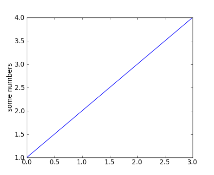
You may be wondering why the x-axis ranges from 0-2 and the y-axis
from 1-3. If you provide a single list or array to the
plot() command, matplotlib assumes it is a
sequence of y values, and automatically generates the x values for
you. Since python ranges start with 0, the default x vector has the
same length as y but starts with 0. Hence the x data are
plot() is a versatile command, and will take an arbitrary number of arguments. For example, to plot x versus y, you can issue the command: plt.clf() plt.plot([1,2,3,4], [1,4,9,16]) Plot() is just the tip of the iceberg for plotting commands and you should study the page of matplotlib screenshots to get a better picture. Clearing the figure with plt.clf() From now on we will assume that you know to clear the figure with clf() before entering commands to make the next plot. For every x, y pair of arguments, there is an optional third argument which is the format string that indicates the color and line type of the plot. The letters and symbols of the format string are from MATLAB, and you concatenate a color string with a line style string. The default format string is ‘b-‘, which is a solid blue line. For example, to plot the above with red circles, you would issue: plt.clf() plt.plot([1,2,3,4], [1,4,9,16], 'ro') plt.axis([0, 6, 0, 20]) 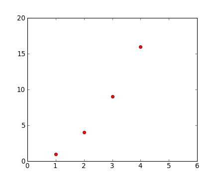
See the plot() documentation for a complete
list of line styles and format strings. The
axis() command in the example above takes a
list of If matplotlib were limited to working with lists, it would be fairly useless for numeric processing. Generally, you will use NumPy arrays. In fact, all sequences are converted to numpy arrays internally. The example below illustrates a plotting several lines with different format styles in one command using arrays: # evenly sampled time at 200ms intervals t = np.arange(0., 5., 0.2) # red dashes, blue squares and green triangles # then filled circle with connecting line plt.clf() plt.plot(t, t, 'r--', t, t**2, 'bs', t, t**3, 'g^') plt.plot(t, t+60, 'o', linestyle='-', color='c') 
Exercise: Make this plot 
Use the plot() documentation to make a plot that looks similar to the one above. Start with: x = [1, 2, 3, 4] y = [3, 2, 3, 1] Click to Show/Hide Solution x = [1, 2, 3, 4] y = [3, 2, 3, 1] plt.clf() plt.plot(x, y, '-.', linewidth=10) plt.plot(x, y, 'H', markeredgecolor='b', markeredgewidth=10, markerfacecolor='r', markersize=40) plt.axis([0, 5, 0, 4]) What are all these icons for?¶The figures are enclosed in a window that looks a little like the following (it depends on the OS and matplotlib backend being used): 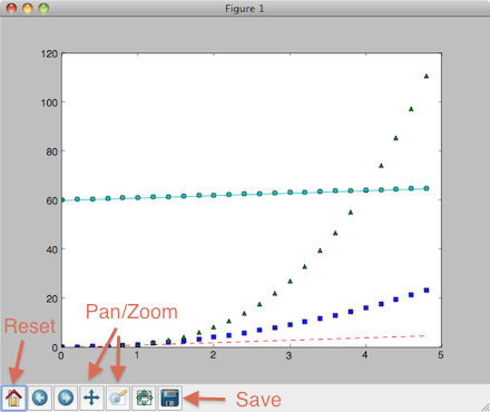
The icons at the bottom of the window allow you to zoom in or out of the plot, pan around, and save the plot as a “hardcopy” format (e.g. PNG, postscript, or PDF). The first icon will reset you to the original axis limits, which comes in quite handy. You can use the close button to close the window, but it is best to use the close() command to avoid memory leaks. Saving the plot¶As discussed above, you can use the GUI to save the plot, but the savefig() command is often more useful, and has many options: plt.savefig('fig.png') plt.savefig('fig.pdf') Note that you can save a figure multiple times (e.g. as different formats). The supported formats depend on the backend being used, but normally include png, pdf, ps, eps and svg: plt.savefig('fig') # creates fig.png (unless you have changed the default format)
plt.savefig('fig.pdf') # creates a PDF file, fig.pdf
plt.savefig('fig', format='svg') # creates a SVG file called fig
plt.savefig('fig.svg', 'format='ps') # creates a PS file called fig.svg (do not do this!)
The default format (used in the first line) can be queried, or changed, by saying: >>> rcParams['savefig.format'] 'png' >>> rcParams['savefig.format'] = 'pdf' >>> plt.savefig('foo') # creates foo.pdf Some common-ish Python errors¶Here’s a couple of errors you may come across: >>> plt.clf <function matplotlib.pyplot.clf> >>> x = np.arange(5) >>> x.size() TypeError: 'int' object is not callable Since For the second case, tarfile.open(fileobj=request.urlopen(url), mode='r|').extractall() Controlling line properties¶What are lines and markers? A matplotlib “line” is a object containing a set of points and various attributes describing how to draw those points. The points are optionally drawn with “markers” and the connections between points can be drawn with various styles of line (including no connecting line at all). Lines have many attributes that you can set: linewidth, dash style, antialiased, etc; see Line2D. There are several ways to set line properties
Important In contrast to old-school plotting where you issue a plot command and the line is immortalized, in matplotlib the lines (and basically everything about the plot) are dynamic objects that can be modified after the fact. Here are the available Line2D properties.
To get a list of settable line properties, call the setp() function with a line or lines as argument: lines = plt.plot([1,2,3]) plt.setp(lines) Detour into Python You may have noticed that in the last workshop we mostly used NumPy arrays like
Some useful functions for controlling plotting¶Here are a few useful functions:
Working with multiple figures and axes¶MATLAB, and matplotlib.pyplot, have the concept of the current figure and the current axes. All plotting commands apply to the current axes. The function gca() returns the current axes (an Axes instance), and gcf() returns the current figure (a Figure instance). Normally, you don’t have to worry about this, because it is all taken care of behind the scenes. Figure, Axes, plot(), and subplot()
Below is a script that illustrates this by creating two figures where the first figure has two subplots: def f(t): """Python function to calculate a decaying sinusoid""" val = np.exp(-t) * np.cos(2*np.pi*t) return val t1 = np.arange(0.0, 5.0, 0.1) t2 = np.arange(0.0, 5.0, 0.02) plt.figure(1) # Make the first figure plt.clf() plt.subplot(2, 1, 1) # 2 rows, 1 column, plot 1 plt.plot(t1, f(t1), 'bo', t2, f(t2), 'k') plt.title('FIGURE 1') plt.text(2, 0.8, 'AXES 211') plt.subplot(2, 1, 2) # 2 rows, 1 column, plot 2 plt.plot(t2, np.cos(2*np.pi*t2), 'r--') plt.text(2, 0.8, 'AXES 212') plt.figure(2) # Make a second figure plt.clf() plt.plot(t2, f(t2), '*') plt.grid() plt.title('FIGURE 2') plt.text(2, 0.8, 'AXES 111')
The first figure() command here is optional because
The subplot() command specifies If you want to place an axes manually, ie, not on a rectangular grid, use the
axes() command, which allows you to specify the location as You can move back to existing subplots, or indeed figures, as shown below: plt.figure(1) # Select the existing first figure plt.subplot(2, 1, 2) # Select the existing subplot 212 plt.plot(t2, np.cos(np.pi*t2), 'g--') # Add a plot to the axes plt.text(0.2, -0.8, 'Back to AXES 212', color='g', size=18) # add a colored label, increasing the font size You can clear the current figure with clf() and the current axes with cla(). If you find this statefulness, annoying, don’t despair, this is just a thin stateful wrapper around an object oriented API, which you can use instead. See the Advanced plotting page for an introduction to this approach, and the then Artist tutorial for the gory details. Figures can be deleted with the close() command: plt.close(2) # Remove the second figure Using close You can use the ‘close button’ provided by the window manager
to remove the figure, but if you do this you must still call
the close() command, to ensure that memory allocated by pyplot
for the figure is released. This is only really an issue for
long-running Working with text¶The text() command can be used to add text in an arbitrary location, and the xlabel(), ylabel() and title() are used to add text in the indicated locations (see Text intro for a more detailed example): mu, sigma = 100, 15 x = np.random.normal(mu, sigma, size=10000) plt.clf() # the histogram of the data histvals, binvals, patches = plt.hist(x, bins=50, normed=True, facecolor='g', alpha=0.75) plt.xlabel('Smarts') plt.ylabel('Probability') plt.title('Histogram of IQ') plt.text(60, .025, r'$\mu=100,\ \sigma=15$') plt.axis([40, 160, 0, 0.03]) plt.grid(True) 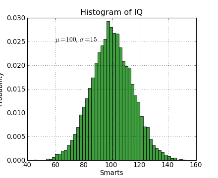
All of the text() commands return an
t = plt.xlabel('my data', fontsize=14, color='red') These properties are covered in more detail in text-properties. Exercise: Overlaying histograms Make an additional normal distribution with a mean of 130. Make a new plot where the two distributions are overlayed. Use a different color and choose the opacities so it looks reasonable. Hint:
Click to Show/Hide Solution plt.clf() x2 = np.random.normal(130, sigma, size=10000) out = plt.hist(x, bins=50, facecolor='g', alpha=0.5) out2 = plt.hist(x2, bins=50, facecolor='r', alpha=0.5) Getting the fonts just right¶The global font properties for various plot elements can be controlled using the rc() function: plt.rc("font", size=10, family='normal', weight='bold') plt.rc("axes", labelsize=10, titlesize=10) plt.rc("xtick", labelsize=10) plt.rc("ytick", labelsize=10) plt.rc("legend", fontsize=10) The inconsistency here is one of the warts in matplotlib. Ironically my favorite way to find these valuable commands is to google “matplotlib makes me hate” which brings up a blog post ranting about the problems with matplotlib. All of the attributes that can be controlled with the rc() command are
listed in See also the Advanced plotting page. Using mathematical expressions in text¶matplotlib accepts TeX equation expressions in any text expression.
For example to write the expression plt.title(r'$\sigma_i=15$') The Annotating text¶The uses of the basic text() command above
place text at an arbitrary position on the Axes. A common use case of
text is to annotate some feature of the plot, and the
annotate() method provides helper
functionality to make annotations easy. In an annotation, there are
two points to consider: the location being annotated represented by
the argument plt.clf() t = np.arange(0.0, 5.0, 0.01) s = np.cos(2*pi*t) lines = plt.plot(t, s, lw=2) plt.annotate('local max', xy=(2, 1), xytext=(3, 1.5), arrowprops=dict(facecolor='black', shrink=0.05)) plt.ylim(-2,2) 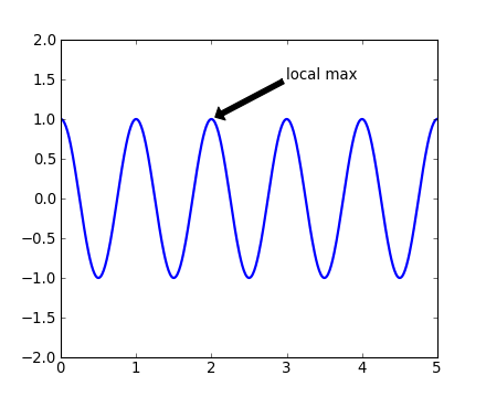
In this basic example, both the Plotting 2-d data¶A deeper tutorial on plotting 2-d image data will have to wait for another day:
Plotting 3-d data¶Matplotlib supports plotting 3-d data through the from mpl_toolkits.mplot3d import Axes3D def randrange(n, vmin, vmax): return (vmax-vmin)*np.random.rand(n) + vmin fig = plt.figure() ax = fig.add_subplot(111, projection='3d') n = 100 for c, m, zl, zh in [('r', 'o', -50, -25), ('b', '^', -30, -5)]: xs = randrange(n, 23, 32) ys = randrange(n, 0, 100) zs = randrange(n, zl, zh) ax.scatter(xs, ys, zs, c=c, marker=m) ax.set_xlabel('X Label') ax.set_ylabel('Y Label') ax.set_zlabel('Z Label') 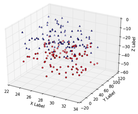
To get more information check out the mplot3d tutorial. Appendix: Pylab and Pyplot and NumPy¶You may see examples that use the matplotlib.pyplot is a collection of command style functions that make matplotlib work like MATLAB. This is just a package module that you can import: import matplotlib.pyplot print(sorted(dir(matplotlib.pyplot))) Likewise pylab is also a module provided by matplotlib that you can import: import pylab This module is a thin wrapper around
There is no magic, and to see for yourself do import matplotlib.pylab matplotlib.pylab?? # prints the source code!! When you do from pylab import * There is one technical detail about GUI event loops and plot window interaction
which makes it useful to use In a lot of documentation examples you will see code like: import matplotlib.pyplot as plt # set plt as alias for matplotlib.pyplot plt.plot([1,2], [3,4]) Now you should understand this is the same See Matplotlib, pylab, and pyplot: how are they related? for a more discussion on the topic. | ||||||||||||||||||||||||||||||||||||||||||||||||||||||||||||||||||||||||||||||||||||
| You are visitor 01402520 — GeezerVison does not store the pages you look up. Best viewed with Netscape Navigator 4.7 or Internet Explorer 6 at 800×600. No cookies required. |


 in the title,
you can write a TeX expression surrounded by dollar signs: