GeezerVison

Support Vector Assertions

Welcome to the 22nd part of our machine learning tutorial series and the next part in our Support Vector Machine section. In this tutorial we will be covering some of the assertions that we're making upon our SVM. Understanding these assertions, some of which will become constraints, will be integral to undertanding both the math and the beauty of the Support Vector Machine.

First, let's take a look at an example "objective" of the SVM. The idea is to take known data, and then the SVM's fitment/training is actually an optimization problem that seeks to find the "best separating" line for the data, known as the decision boundary. Something like this: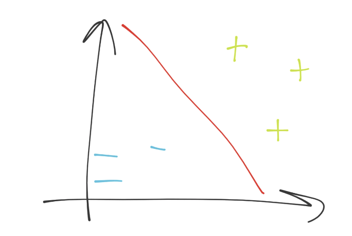

We're in 2D space, so the separating hyperplane (decision boundary) just looks like a simple line (the red line). This decision boundary is separating the blue minus group from the green plus sign group. Next, if we were to put a point anywhere on this graph, we'd just do a simple check to see which side of the separating hyperplane it was on, and boom we have our answer. How easy is that?! Piece of cake indeed...if we could just stay in 2D. What are the dimensions in our case? Each dimension is a feature, and all of the dimensions make up our featureset. Thus, we might have a simple line, which is super easy. We could solve this with linear algebra with no trouble at all. What about when we have 63 features, so 63 dimensions?

It's not so clear at that point, no different than when we suddenly have more than 2 dimensions with Pythagorean's theorm. Fine, we move to vectorspace! Poof, we're in vector space, and now we've got an unknown featureset, noted by vector u. Then, we have another vector perpendicular to the decision boundary, vector w. It might look like: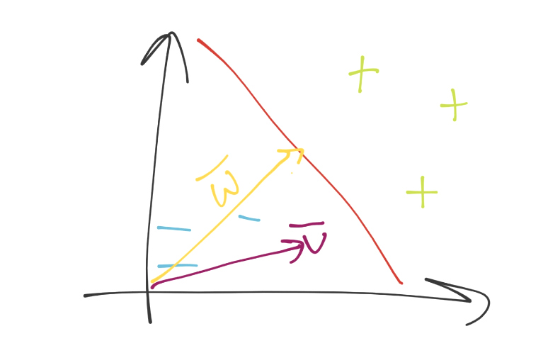

Now what? We can visually tell what the deal is, but how would we know mathematically. Again, remember you need a method that will work in both 2 dimensions and 5,902. We can just project vector u onto vector w, add some bias (b), and then see if the value is above or below 0 for the class.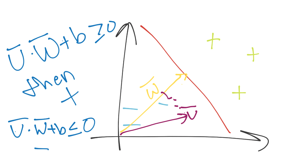

Great, except for the whole thing where we have no idea what w is and what b is.

The plot thickens.

We have two unknown variables still, and I am here to bring the bad news: we have to derive them. Immediately, this should send off red flags regarding optimization. There are an infinite number of w's and b's that might satisfy our equation, but we also know that we have a sort of constraint already defined logically in our heads: we want the "best" separating hyperplane. The best separating hyperplane is the one with the most width between the data it is separating. We can probably guess that's going to play a part in the optimization of w and b. To begin, we're going to have to set some actual mathematical constraints.

So far, we've just seen the separating hyperplane, but the separating hyperlane is actually in between two other hyperplanes. The other hyperplanes are going through what are called the support vectors, which are the featuresets (datapoints on the graph), which, if moved, would have an impact on the best separating hyperplane.

Because these support vectors have such a major impact, we're going to set a constant value to them. Recall the classification function was just 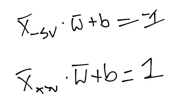sign(x.w + b) (the period signals the dot product). What if x.w+b is 0? This means we're right on the decision boundary. Otherwise, if it is above 0, then we have a positive class. If below zero, it's a negative class. We're going to take advantage of this, and then go a step further and suggest that if x.w+b is 1, then this is a positive support vector. If x.w+b is -1, then this is a negative support vector. Later, an unknown might be -.52. It's still a negative class, even though it's not beyond the -1 that is the support vector mark. We're simply using support vectors to help us pick the best separating hyperplane, that is their only use. In written form, we're asserting that:

What that says is, on the first line, we have the X-sub-negative-support-vector (this is any featureset that IS a negative support vector) dotted with vector w + b is equal to -1. We're just asserting this. We do the same thing for the positive support vector: X-sub-positive-support-vector dotted with vector w + b is positive one. Again, we're just stating this, there's no real proof, we're just saying this is the case. Now, we're going to bring in a new value, Yi (y sub i):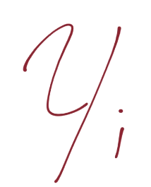

Just like y is our "class" value in Python code, it is here too.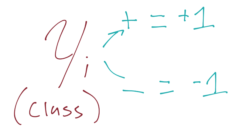

We're going to introduce this to our previous assertion, which, if you recall was for the value of the positive and negative support vectors x.w+b=1 for positive support vector and x.w+b=-1 for a negative support vector. We are going to multiply our original assertion:

By this new 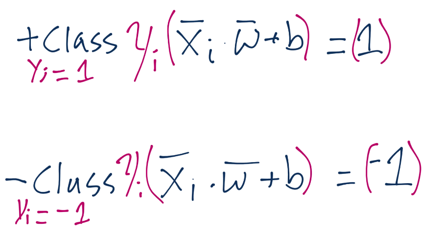Yi value, which, again, is just -1 or 1 (depending on whether or not the class is a -1 or a 1). When we multiply the original assertion, we have to multiply both sides by Yi, which becomes:

We'll leave just the notation of 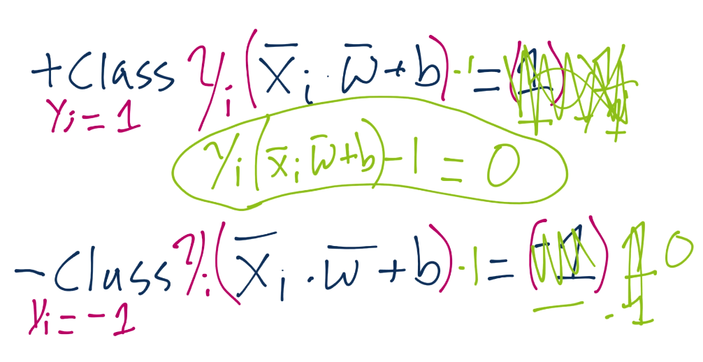Yi on the left side, but we'll actually apply it to the right-side (which is 1 or -1). Doing this means for the positive support vectors, we'd have 1 x 1, so one. For negative support vectors, we'd have -1 x -1, so again we have 1. We can set both equations equal to zero, subtracting 1 from both sides, and we have the exact same equation, Yi(Xi.w+b)-1 = 0:

Now we have our constraint, which is what we're going to be talking more about in the next tutorial.

The next tutorial: