GeezerVison is showing scikit-learn.org — Analysis of the convergence of penalized logistic regression models
Note
Go to the end
to download the full example code or to run this example in your browser via JupyterLite or Binder.
Analysis of the convergence of penalized logistic regression models#
The purpose of this example is three-fold:
Demonstrate registering a ScoringMonitor on the logistic
regression step of a pipeline nested inside
GridSearchCV. Show how to plot the metric values collected at each iteration of each fit
of the logistic regression model during the grid search and analyze the
convergence of the model for each hyperparameter combination. Show how the monitoring of diverse scoring metrics can inform us about the
quality of the model and the trade-off between refinement and calibration.
# Authors: The scikit-learn developers
# SPDX-License-Identifier: BSD-3-Clause
Setup#
Let’s first define the pipeline and the grid search. Here we register a
ScoringMonitor callback on the logistic regression model to monitor
the scores at each iteration of the L-BFGS solver.
We reuse the same scoring metrics for the grid search itself and use the D²
log-loss as the primary metric to select the best hyperparameter combination.
import matplotlib.pyplot as plt
import numpy as np
import pandas as pd

from sklearn.callback import ProgressBar, ScoringMonitor
from sklearn.datasets import make_classification
from sklearn.linear_model import LogisticRegression
from sklearn.model_selection import GridSearchCV
from sklearn.pipeline import make_pipeline
from sklearn.preprocessing import StandardScaler

X, y = make_classification(
    n_samples=1000, n_features=100, n_classes=10, n_informative=30, random_state=42
)

scoring_metrics = ["d2_log_loss_score", "accuracy", "average_precision"]
scoring_monitor = ScoringMonitor(scoring=scoring_metrics)
model = make_pipeline(
    StandardScaler(),
    LogisticRegression(solver="lbfgs", max_iter=1000).set_callbacks(scoring_monitor),
)

param_grid = {
    "standardscaler__with_std": [True, False],
    "logisticregression__C": np.geomspace(0.01, 100, 3),
}

grid_search = GridSearchCV(
    model,
    param_grid,
    cv=5,
    scoring=scoring_metrics,
    n_jobs=2,
    error_score="raise",
    refit=scoring_metrics[0],
)
Let’s fit the grid search with the auto-propagating progress bar callback.
Feel free to set max_propagation_depth=3 in the ProgressBar constructor to
get a more detailed output by displaying the progress bars for the pipeline,
the standard scaler and the logistic regression.
GridSearchCV - fit                                                 ━━━ 100% 0:0…
  GridSearchCV - search #0                                         ━━━ 100% 0:0…
    GridSearchCV - candidate-split-evaluation | Pipeline - fit #0  ━━━ 100% 0:0…
    GridSearchCV - candidate-split-evaluation | Pipeline - fit #1  ━━━ 100% 0:0…
    GridSearchCV - candidate-split-evaluation | Pipeline - fit #2  ━━━ 100% 0:0…
    GridSearchCV - candidate-split-evaluation | Pipeline - fit #3  ━━━ 100% 0:0…
    GridSearchCV - candidate-split-evaluation | Pipeline - fit #4  ━━━ 100% 0:0…
    GridSearchCV - candidate-split-evaluation | Pipeline - fit #5  ━━━ 100% 0:0…
    GridSearchCV - candidate-split-evaluation | Pipeline - fit #6  ━━━ 100% 0:0…
    GridSearchCV - candidate-split-evaluation | Pipeline - fit #7  ━━━ 100% 0:0…
    GridSearchCV - candidate-split-evaluation | Pipeline - fit #8  ━━━ 100% 0:0…
    GridSearchCV - candidate-split-evaluation | Pipeline - fit #9  ━━━ 100% 0:0…
    GridSearchCV - candidate-split-evaluation | Pipeline - fit #10 ━━━ 100% 0:0…
    GridSearchCV - candidate-split-evaluation | Pipeline - fit #11 ━━━ 100% 0:0…
    GridSearchCV - candidate-split-evaluation | Pipeline - fit #12 ━━━ 100% 0:0…
    GridSearchCV - candidate-split-evaluation | Pipeline - fit #13 ━━━ 100% 0:0…
    GridSearchCV - candidate-split-evaluation | Pipeline - fit #14 ━━━ 100% 0:0…
    GridSearchCV - candidate-split-evaluation | Pipeline - fit #15 ━━━ 100% 0:0…
    GridSearchCV - candidate-split-evaluation | Pipeline - fit #16 ━━━ 100% 0:0…
    GridSearchCV - candidate-split-evaluation | Pipeline - fit #17 ━━━ 100% 0:0…
    GridSearchCV - candidate-split-evaluation | Pipeline - fit #18 ━━━ 100% 0:0…
    GridSearchCV - candidate-split-evaluation | Pipeline - fit #19 ━━━ 100% 0:0…
    GridSearchCV - candidate-split-evaluation | Pipeline - fit #20 ━━━ 100% 0:0…
    GridSearchCV - candidate-split-evaluation | Pipeline - fit #21 ━━━ 100% 0:0…
    GridSearchCV - candidate-split-evaluation | Pipeline - fit #22 ━━━ 100% 0:0…
    GridSearchCV - candidate-split-evaluation | Pipeline - fit #23 ━━━ 100% 0:0…
    GridSearchCV - candidate-split-evaluation | Pipeline - fit #24 ━━━ 100% 0:0…
    GridSearchCV - candidate-split-evaluation | Pipeline - fit #25 ━━━ 100% 0:0…
    GridSearchCV - candidate-split-evaluation | Pipeline - fit #26 ━━━ 100% 0:0…
    GridSearchCV - candidate-split-evaluation | Pipeline - fit #27 ━━━ 100% 0:0…
    GridSearchCV - candidate-split-evaluation | Pipeline - fit #28 ━━━ 100% 0:0…
    GridSearchCV - candidate-split-evaluation | Pipeline - fit #29 ━━━ 100% 0:0…
  GridSearchCV - refit-with-best-params | Pipeline - fit #1        ━━━ 100% 0:0…
GridSearchCV(cv=5, error_score='raise',
             estimator=Pipeline(steps=[('standardscaler', StandardScaler()),
                                       ('logisticregression',
                                        LogisticRegression(max_iter=1000))]),
             n_jobs=2,
             param_grid={'logisticregression__C': array([1.e-02, 1.e+00, 1.e+02]),
                         'standardscaler__with_std': [True, False]},
             refit='d2_log_loss_score',
             scoring=['d2_log_loss_score', 'accuracy', 'average_precision'])
In a Jupyter environment, please rerun this cell to show the HTML representation or trust the notebook.
On GitHub, the HTML representation is unable to render, please try loading this page with nbviewer.org.
Parameters
|
estimator
estimator: estimator object
This is assumed to implement the scikit-learn estimator interface.
Either estimator needs to provide a ``score`` function,
or ``scoring`` must be passed.
|
Pipeline(step..._iter=1000))]) |
|
param_grid
param_grid: dict or list of dictionaries
Dictionary with parameters names (`str`) as keys and lists of
parameter settings to try as values, or a list of such
dictionaries, in which case the grids spanned by each dictionary
in the list are explored. This enables searching over any sequence
of parameter settings.
|
{'logisticregression__C': array([1.e-02...e+00, 1.e+02]), 'standardscaler__with_std': [True, False]} |
|
scoring
scoring: str, callable, list, tuple or dict, default=None
Strategy to evaluate the performance of the cross-validated model on
the test set.
If `scoring` represents a single score, one can use:
- a single string (see :ref:`scoring_string_names`);
- a callable (see :ref:`scoring_callable`) that returns a single value;
- `None`, the `estimator`'s
:ref:`default evaluation criterion <scoring_api_overview>` is used.
If `scoring` represents multiple scores, one can use:
- a list or tuple of unique strings;
- a callable returning a dictionary where the keys are the metric
names and the values are the metric scores;
- a dictionary with metric names as keys and callables as values.
See :ref:`multimetric_grid_search` for an example.
|
['d2_log_loss_score', 'accuracy', ...] |
|
n_jobs
n_jobs: int, default=None
Number of jobs to run in parallel.
``None`` means 1 unless in a :obj:`joblib.parallel_backend` context.
``-1`` means using all processors. See :term:`Glossary <n_jobs>`
for more details.
.. versionchanged:: v0.20
`n_jobs` default changed from 1 to None
|
2 |
|
refit
refit: bool, str, or callable, default=True
Refit an estimator using the best found parameters on the whole
dataset.
For multiple metric evaluation, this needs to be a `str` denoting the
scorer that would be used to find the best parameters for refitting
the estimator at the end.
Where there are considerations other than maximum score in
choosing a best estimator, ``refit`` can be set to a function which
returns the selected ``best_index_`` given ``cv_results_``. In that
case, the ``best_estimator_`` and ``best_params_`` will be set
according to the returned ``best_index_`` while the ``best_score_``
attribute will not be available.
The refitted estimator is made available at the ``best_estimator_``
attribute and permits using ``predict`` directly on this
``GridSearchCV`` instance.
Also for multiple metric evaluation, the attributes ``best_index_``,
``best_score_`` and ``best_params_`` will only be available if
``refit`` is set and all of them will be determined w.r.t this specific
scorer.
See ``scoring`` parameter to know more about multiple metric
evaluation.
See :ref:`sphx_glr_auto_examples_model_selection_plot_grid_search_digits.py`
to see how to design a custom selection strategy using a callable
via `refit`.
See :ref:`this example
<sphx_glr_auto_examples_model_selection_plot_grid_search_refit_callable.py>`
for an example of how to use ``refit=callable`` to balance model
complexity and cross-validated score.
.. versionchanged:: 0.20
Support for callable added.
|
'd2_log_loss_score' |
|
cv
cv: int, cross-validation generator or an iterable, default=None
Determines the cross-validation splitting strategy.
Possible inputs for cv are:
- None, to use the default 5-fold cross validation,
- integer, to specify the number of folds in a `(Stratified)KFold`,
- :term:`CV splitter`,
- an iterable yielding (train, test) splits as arrays of indices.
For integer/None inputs, if the estimator is a classifier and ``y`` is
either binary or multiclass, :class:`StratifiedKFold` is used. In all
other cases, :class:`KFold` is used. These splitters are instantiated
with `shuffle=False` so the splits will be the same across calls.
Refer :ref:`User Guide <cross_validation>` for the various
cross-validation strategies that can be used here.
.. versionchanged:: 0.22
``cv`` default value if None changed from 3-fold to 5-fold.
|
5 |
|
error_score
error_score: 'raise' or numeric, default=np.nan
Value to assign to the score if an error occurs in estimator fitting.
If set to 'raise', the error is raised. If a numeric value is given,
FitFailedWarning is raised. This parameter does not affect the refit
step, which will always raise the error.
|
'raise' |
|
verbose
verbose: int, default=0
Controls the verbosity of information printed during fitting, with higher
values yielding more detailed logging.
- 0 : no messages are printed;
- >=1 : summary of the total number of fits;
- >=2 : computation time for each fold and parameter candidate;
- >=3 : fold indices and scores;
- >=10 : parameter candidate indices and START messages before each fit.
|
0 |
|
pre_dispatch
pre_dispatch: int, or str, default='2*n_jobs'
Controls the number of jobs that get dispatched during parallel
execution. Reducing this number can be useful to avoid an
explosion of memory consumption when more jobs get dispatched
than CPUs can process. This parameter can be:
- None, in which case all the jobs are immediately created and spawned. Use
this for lightweight and fast-running jobs, to avoid delays due to on-demand
spawning of the jobs
- An int, giving the exact number of total jobs that are spawned
- A str, giving an expression as a function of n_jobs, as in '2*n_jobs'
|
'2*n_jobs' |
|
return_train_score
return_train_score: bool, default=False
If ``False``, the ``cv_results_`` attribute will not include training
scores.
Computing training scores is used to get insights on how different
parameter settings impact the overfitting/underfitting trade-off.
However computing the scores on the training set can be computationally
expensive and is not strictly required to select the parameters that
yield the best generalization performance.
.. versionadded:: 0.19
.. versionchanged:: 0.21
Default value was changed from ``True`` to ``False``
|
False |
Fitted attributes
| Name |
Type |
Value |
best_estimator_
best_estimator_: estimator
Estimator that was chosen by the search, i.e. estimator
which gave highest score (or smallest loss if specified)
on the left out data. Not available if ``refit=False``.
See ``refit`` parameter for more information on allowed values.
|
Pipeline |
Pipeline(step..._iter=1000))]) |
best_index_
best_index_: int
The index (of the ``cv_results_`` arrays) which corresponds to the best
candidate parameter setting.
The dict at ``search.cv_results_['params'][search.best_index_]`` gives
the parameter setting for the best model, that gives the highest
mean score (``search.best_score_``).
For multi-metric evaluation, this is present only if ``refit`` is
specified.
|
int64 |
np.int64(1) |
best_params_
best_params_: dict
Parameter setting that gave the best results on the hold out data.
For multi-metric evaluation, this is present only if ``refit`` is
specified.
|
dict |
{'lo..._C': np.float64(0.01), 'st...td': False} |
best_score_
best_score_: float
Mean cross-validated score of the best_estimator
For multi-metric evaluation, this is present only if ``refit`` is
specified.
This attribute is not available if ``refit`` is a function.
|
float64 |
0.1706 |
classes_
classes_: ndarray of shape (n_classes,)
The classes labels. This is present only if ``refit`` is specified and
the underlying estimator is a classifier.
|
ndarray[int64](10,) |
[0,1,2,...,7,8,9] |
cv_results_
cv_results_: dict of numpy (masked) ndarrays
A dict with keys as column headers and values as columns, that can be
imported into a pandas ``DataFrame``.
For instance the below given table
+------------+-----------+------------+-----------------+---+---------+
|param_kernel|param_gamma|param_degree|split0_test_score|...|rank_t...|
+============+===========+============+=================+===+=========+
| 'poly' | -- | 2 | 0.80 |...| 2 |
+------------+-----------+------------+-----------------+---+---------+
| 'poly' | -- | 3 | 0.70 |...| 4 |
+------------+-----------+------------+-----------------+---+---------+
| 'rbf' | 0.1 | -- | 0.80 |...| 3 |
+------------+-----------+------------+-----------------+---+---------+
| 'rbf' | 0.2 | -- | 0.93 |...| 1 |
+------------+-----------+------------+-----------------+---+---------+
will be represented by a ``cv_results_`` dict of::
{
'param_kernel': masked_array(data = ['poly', 'poly', 'rbf', 'rbf'],
mask = [False False False False]...)
'param_gamma': masked_array(data = [-- -- 0.1 0.2],
mask = [ True True False False]...),
'param_degree': masked_array(data = [2.0 3.0 -- --],
mask = [False False True True]...),
'split0_test_score' : [0.80, 0.70, 0.80, 0.93],
'split1_test_score' : [0.82, 0.50, 0.70, 0.78],
'mean_test_score' : [0.81, 0.60, 0.75, 0.85],
'std_test_score' : [0.01, 0.10, 0.05, 0.08],
'rank_test_score' : [2, 4, 3, 1],
'split0_train_score' : [0.80, 0.92, 0.70, 0.93],
'split1_train_score' : [0.82, 0.55, 0.70, 0.87],
'mean_train_score' : [0.81, 0.74, 0.70, 0.90],
'std_train_score' : [0.01, 0.19, 0.00, 0.03],
'mean_fit_time' : [0.73, 0.63, 0.43, 0.49],
'std_fit_time' : [0.01, 0.02, 0.01, 0.01],
'mean_score_time' : [0.01, 0.06, 0.04, 0.04],
'std_score_time' : [0.00, 0.00, 0.00, 0.01],
'params' : [{'kernel': 'poly', 'degree': 2}, ...],
}
For an example of visualization and interpretation of GridSearch results,
see :ref:`sphx_glr_auto_examples_model_selection_plot_grid_search_stats.py`.
NOTE
The key ``'params'`` is used to store a list of parameter
settings dicts for all the parameter candidates.
The ``mean_fit_time``, ``std_fit_time``, ``mean_score_time`` and
``std_score_time`` are all in seconds.
For multi-metric evaluation, the scores for all the scorers are
available in the ``cv_results_`` dict at the keys ending with that
scorer's name (``'_<scorer_name>'``) instead of ``'_score'`` shown
above. ('split0_test_precision', 'mean_train_precision' etc.)
|
dict |
{'me...me': array([0.2121... 3.88371768]), 'me...me': array([0.0190... 0.01351433]), 'me...cy': array([0.296,...0.26 , 0.258]), 'me...on': array([0.2980... 0.26786657]), ...} |
multimetric_
multimetric_: bool
Whether or not the scorers compute several metrics.
|
bool |
True |
n_features_in_
n_features_in_: int
Number of features seen during :term:`fit`. Only defined if
`best_estimator_` is defined (see the documentation for the `refit`
parameter for more details) and that `best_estimator_` exposes
`n_features_in_` when fit.
.. versionadded:: 0.24
|
int |
100 |
n_splits_
n_splits_: int
The number of cross-validation splits (folds/iterations).
|
int |
5 |
refit_time_
refit_time_: float
Seconds used for refitting the best model on the whole dataset.
This is present only if ``refit`` is not False.
.. versionadded:: 0.20
|
float |
1.074 |
scorer_
scorer_: function or a dict
Scorer function used on the held out data to choose the best
parameters for the model.
For multi-metric evaluation, this attribute holds the validated
``scoring`` dict which maps the scorer key to the scorer callable.
|
dict |
{'ac...cy': make_scorer(a...hod='predict'), 'av...on': make_scorer(a...edict_proba')), 'd2...re': make_scorer(d...redict_proba')} |
best_estimator_: Pipeline
Fitted attributes
| Name |
Type |
Value |
mean_
mean_: ndarray of shape (n_features,) or None
The mean value for each feature in the training set.
Equal to ``None`` when ``with_mean=False`` and ``with_std=False``.
|
ndarray[float64](100,) |
[-0.1 , 0.05, 0. ,..., 0.06,-0. , 0.3 ] |
n_features_in_
n_features_in_: int
Number of features seen during :term:`fit`.
.. versionadded:: 0.24
|
int |
100 |
n_samples_seen_
n_samples_seen_: int or ndarray of shape (n_features,)
The number of samples processed by the estimator for each feature.
If there are no missing samples, the ``n_samples_seen`` will be an
integer, otherwise it will be an array of dtype int. If
`sample_weights` are used it will be a float (if no missing data)
or an array of dtype float that sums the weights seen so far.
Will be reset on new calls to fit, but increments across
``partial_fit`` calls.
|
float64 |
1000 |
scale_
scale_: ndarray of shape (n_features,) or None
Per feature relative scaling of the data to achieve zero mean and unit
variance. Generally this is calculated using `np.sqrt(var_)`. If a
variance is zero, we can't achieve unit variance, and the data is left
as-is, giving a scaling factor of 1. `scale_` is equal to `None`
when `with_std=False`.
.. versionadded:: 0.17
*scale_*
|
NoneType |
None |
var_
var_: ndarray of shape (n_features,) or None
The variance for each feature in the training set. Used to compute
`scale_`. Equal to ``None`` when ``with_mean=False`` and
``with_std=False``.
|
NoneType |
None |
100 features
| x0 |
| x1 |
| x2 |
| x3 |
| x4 |
| x5 |
| x6 |
| x7 |
| x8 |
| x9 |
| x10 |
| x11 |
| x12 |
| x13 |
| x14 |
| x15 |
| x16 |
| x17 |
| x18 |
| x19 |
| x20 |
| x21 |
| x22 |
| x23 |
| x24 |
| x25 |
| x26 |
| x27 |
| x28 |
| x29 |
| x30 |
| x31 |
| x32 |
| x33 |
| x34 |
| x35 |
| x36 |
| x37 |
| x38 |
| x39 |
| x40 |
| x41 |
| x42 |
| x43 |
| x44 |
| x45 |
| x46 |
| x47 |
| x48 |
| x49 |
| x50 |
| x51 |
| x52 |
| x53 |
| x54 |
| x55 |
| x56 |
| x57 |
| x58 |
| x59 |
| x60 |
| x61 |
| x62 |
| x63 |
| x64 |
| x65 |
| x66 |
| x67 |
| x68 |
| x69 |
| x70 |
| x71 |
| x72 |
| x73 |
| x74 |
| x75 |
| x76 |
| x77 |
| x78 |
| x79 |
| x80 |
| x81 |
| x82 |
| x83 |
| x84 |
| x85 |
| x86 |
| x87 |
| x88 |
| x89 |
| x90 |
| x91 |
| x92 |
| x93 |
| x94 |
| x95 |
| x96 |
| x97 |
| x98 |
| x99 |
Parameters
|
C
C: float, default=1.0
Inverse of regularization strength; must be a positive float.
Like in support vector machines, smaller values specify stronger
regularization. `C=np.inf` results in unpenalized logistic regression.
For a visual example on the effect of tuning the `C` parameter
with an L1 penalty, see:
:ref:`sphx_glr_auto_examples_linear_model_plot_logistic_path.py`.
|
np.float64(0.01) |
|
max_iter
max_iter: int, default=100
Maximum number of iterations taken for the solvers to converge.
|
1000 |
|
penalty
penalty: {'l1', 'l2', 'elasticnet', None}, default='l2'
Specify the norm of the penalty:
- `None`: no penalty is added;
- `'l2'`: add an L2 penalty term and it is the default choice;
- `'l1'`: add an L1 penalty term;
- `'elasticnet'`: both L1 and L2 penalty terms are added.
.. warning::
Some penalties may not work with some solvers. See the parameter
`solver` below, to know the compatibility between the penalty and
solver.
.. versionadded:: 0.19
l1 penalty with SAGA solver (allowing 'multinomial' + L1)
.. deprecated:: 1.8
`penalty` was deprecated in version 1.8 and will be removed in 1.10.
Use `l1_ratio` and `C` instead. `l1_ratio=0` for `penalty='l2'`,
`l1_ratio=1` for `penalty='l1'`, `l1_ratio` set to any float between 0 and 1
for `penalty='elasticnet'`, and `C=np.inf` for `penalty=None`.
|
'deprecated' |
|
l1_ratio
l1_ratio: float, default=0.0
The Elastic-Net mixing parameter, with `0 <= l1_ratio <= 1`. Setting
`l1_ratio=1` gives a pure L1-penalty, setting `l1_ratio=0` a pure L2-penalty.
Any value between 0 and 1 gives an Elastic-Net penalty of the form
`l1_ratio * L1 + (1 - l1_ratio) * L2`.
.. warning::
Certain values of `l1_ratio`, i.e. some penalties, may not work with some
solvers. See the parameter `solver` below, to know the compatibility between
the penalty and solver.
.. versionchanged:: 1.8
Default value changed from None to 0.0.
.. deprecated:: 1.8
`None` is deprecated and will be removed in version 1.10. Always use
`l1_ratio` to specify the penalty type.
|
0.0 |
|
dual
dual: bool, default=False
Dual (constrained) or primal (regularized, see also
:ref:`this equation <regularized-logistic-loss>`) formulation. Dual formulation
is only implemented for l2 penalty with liblinear solver. Prefer `dual=False`
when n_samples > n_features.
|
False |
|
tol
tol: float, default=1e-4
Tolerance for stopping criteria.
|
0.0001 |
|
fit_intercept
fit_intercept: bool, default=True
Specifies if a constant (a.k.a. bias or intercept) should be
added to the decision function.
|
True |
|
intercept_scaling
intercept_scaling: float, default=1
Useful only when the solver `liblinear` is used
and `self.fit_intercept` is set to `True`. In this case, `x` becomes
`[x, self.intercept_scaling]`,
i.e. a "synthetic" feature with constant value equal to
`intercept_scaling` is appended to the instance vector.
The intercept becomes
``intercept_scaling * synthetic_feature_weight``.
.. note::
The synthetic feature weight is subject to L1 or L2
regularization as all other features.
To lessen the effect of regularization on synthetic feature weight
(and therefore on the intercept) `intercept_scaling` has to be increased.
|
1 |
|
class_weight
class_weight: dict or 'balanced', default=None
Weights associated with classes in the form ``{class_label: weight}``.
If not given, all classes are supposed to have weight one.
The "balanced" mode uses the values of y to automatically adjust
weights inversely proportional to class frequencies in the input data
as ``n_samples / (n_classes * np.bincount(y))``.
Note that these weights will be multiplied with sample_weight (passed
through the fit method) if sample_weight is specified.
.. versionadded:: 0.17
*class_weight='balanced'*
|
None |
|
random_state
random_state: int, RandomState instance, default=None
Only used for `solver` == 'sag', 'saga' or 'liblinear' to shuffle the
data. It has no effect on the other solvers.
See :term:`Glossary <random_state>` for details.
|
None |
|
solver
solver: {'lbfgs', 'liblinear', 'newton-cg', 'newton-cholesky', 'sag', 'saga'}, default='lbfgs'
Algorithm to use in the optimization problem. Default is 'lbfgs'.
To choose a solver, you might want to consider the following aspects:
- 'lbfgs' is a good default solver because it works reasonably well for a wide
class of problems.
- For :term:`multiclass` problems (`n_classes >= 3`), all solvers except
'liblinear' minimize the full multinomial loss, 'liblinear' will raise an
error.
- 'newton-cholesky' is a good choice for
`n_samples` >> `n_features * n_classes`, especially with one-hot encoded
categorical features with rare categories. Be aware that the memory usage
of this solver has a quadratic dependency on `n_features * n_classes`
because it explicitly computes the full Hessian matrix.
- For small datasets, 'liblinear' is a good choice, whereas 'sag'
and 'saga' are faster for large ones;
- 'liblinear' can only handle binary classification by default. To apply a
one-versus-rest scheme for the multiclass setting one can wrap it with the
:class:`~sklearn.multiclass.OneVsRestClassifier`.
.. warning::
The choice of the algorithm depends on the penalty chosen (`l1_ratio=0`
for L2-penalty, `l1_ratio=1` for L1-penalty and `0 < l1_ratio < 1` for
Elastic-Net) and on (multinomial) multiclass support:
================= ======================== ======================
solver l1_ratio multinomial multiclass
================= ======================== ======================
'lbfgs' l1_ratio=0 yes
'liblinear' l1_ratio=1 or l1_ratio=0 no
'newton-cg' l1_ratio=0 yes
'newton-cholesky' l1_ratio=0 yes
'sag' l1_ratio=0 yes
'saga' 0<=l1_ratio<=1 yes
================= ======================== ======================
.. note::
'sag' and 'saga' fast convergence is only guaranteed on features
with approximately the same scale. You can preprocess the data with
a scaler from :mod:`sklearn.preprocessing`.
.. seealso::
Refer to the :ref:`User Guide <Logistic_regression>` for more
information regarding :class:`LogisticRegression` and more specifically the
:ref:`Table <logistic_regression_solvers>`
summarizing solver/penalty supports.
.. versionadded:: 0.17
Stochastic Average Gradient (SAG) descent solver. Multinomial support in
version 0.18.
.. versionadded:: 0.19
SAGA solver.
.. versionchanged:: 0.22
The default solver changed from 'liblinear' to 'lbfgs' in 0.22.
.. versionadded:: 1.2
newton-cholesky solver. Multinomial support in version 1.6.
|
'lbfgs' |
|
verbose
verbose: int, default=0
For the liblinear and lbfgs solvers set verbose to any positive
number for verbosity.
|
0 |
|
warm_start
warm_start: bool, default=False
When set to True, reuse the solution of the previous call to fit as
initialization, otherwise, just erase the previous solution.
Useless for liblinear solver. See :term:`the Glossary <warm_start>`.
.. versionadded:: 0.17
*warm_start* to support *lbfgs*, *newton-cg*, *sag*, *saga* solvers.
|
False |
|
n_jobs
n_jobs: int, default=None
Does not have any effect.
.. deprecated:: 1.8
`n_jobs` is deprecated in version 1.8 and will be removed in 1.10.
|
None |
Fitted attributes
| Name |
Type |
Value |
classes_
classes_: ndarray of shape (n_classes, )
A list of class labels known to the classifier.
|
ndarray[int64](10,) |
[0,1,2,...,7,8,9] |
coef_
coef_: ndarray or CSR matrix of shape (1, n_features) or (n_classes, n_features)
Coefficients of the features in the decision function.
`coef_` is of shape (1, n_features) when the given problem is binary.
By default, it will be created as a dense array, but can be turned to
sparse (CSR format) through :meth:`sparsify` (which can be beneficial
under L1 regularization when many coefficients are zero), and back to
dense through :meth:`densify`.
|
ndarray[float64](10, 100) |
[[ 0.14,-0. , 0.06,..., 0.01, 0. ,-0. ],
[ 0.01, 0.04, 0.01,..., 0.02,-0.03, 0.01],
[-0.11,-0.04, 0.06,...,-0.06, 0.06, 0. ],
...,
[-0.06, 0.05, 0.04,...,-0.07, 0.03, 0.02],
[-0.03, 0. ,-0.05,..., 0.04,-0.06,-0.14],
[-0.04,-0.05, 0. ,..., 0.03,-0. , 0.05]] |
intercept_
intercept_: ndarray of shape (1,) or (n_classes,)
Intercept (a.k.a. bias) added to the decision function.
If `fit_intercept` is set to False, the intercept is set to zero.
`intercept_` is of shape (1,) when the given problem is binary.
|
ndarray[float64](10,) |
[-0. , 0.23,-0.15,..., 0.13,-0.07,-0.18] |
n_features_in_
n_features_in_: int
Number of features seen during :term:`fit`.
.. versionadded:: 0.24
|
int |
100 |
n_iter_
n_iter_: ndarray of shape (1, )
Actual number of iterations for all classes.
.. versionchanged:: 0.20
In SciPy <= 1.0.0 the number of lbfgs iterations may exceed
``max_iter``. ``n_iter_`` will now report at most ``max_iter``.
|
ndarray[int32](1,) |
[77] |
We use a grid search with 3 values for the regularization parameter C and
2 values for the standardization of the features resulting in 6 parameter
combinations.
Since we use 5-fold cross-validation (cv=5), we will have 5 fits of the
logistic regression model for each parameter combination resulting in 30 fits
as subtasks of the “search” fit task.
In addition, the grid search performs a final refit on the full dataset with
the best hyperparameter combination found during the grid search. This is
visible as the “refit-with-best-params” task in the output above.
Consolidation of the grid search results#
Let’s look at the results of the grid search.
cv_results = pd.DataFrame(grid_search.cv_results_)
cv_results.sort_values(by="rank_test_d2_log_loss_score", ascending=True)
|
mean_fit_time |
std_fit_time |
mean_score_time |
std_score_time |
param_logisticregression__C |
param_standardscaler__with_std |
params |
split0_test_d2_log_loss_score |
split1_test_d2_log_loss_score |
split2_test_d2_log_loss_score |
split3_test_d2_log_loss_score |
split4_test_d2_log_loss_score |
mean_test_d2_log_loss_score |
std_test_d2_log_loss_score |
rank_test_d2_log_loss_score |
split0_test_accuracy |
split1_test_accuracy |
split2_test_accuracy |
split3_test_accuracy |
split4_test_accuracy |
mean_test_accuracy |
std_test_accuracy |
rank_test_accuracy |
split0_test_average_precision |
split1_test_average_precision |
split2_test_average_precision |
split3_test_average_precision |
split4_test_average_precision |
mean_test_average_precision |
std_test_average_precision |
rank_test_average_precision |
| 1 |
1.477605 |
0.081582 |
0.014521 |
0.004147 |
0.01 |
False |
{'logisticregression__C': 0.01, 'standardscale... |
0.135960 |
0.167780 |
0.189062 |
0.173567 |
0.186634 |
0.170601 |
0.019051 |
1 |
0.285 |
0.330 |
0.330 |
0.355 |
0.305 |
0.321 |
0.023958 |
1 |
0.319819 |
0.309708 |
0.360697 |
0.323126 |
0.340503 |
0.330771 |
0.017957 |
1 |
| 0 |
0.212196 |
0.032597 |
0.019046 |
0.012373 |
0.01 |
True |
{'logisticregression__C': 0.01, 'standardscale... |
0.125785 |
0.112817 |
0.129538 |
0.127723 |
0.140616 |
0.127296 |
0.008883 |
2 |
0.290 |
0.275 |
0.315 |
0.320 |
0.280 |
0.296 |
0.018276 |
2 |
0.293645 |
0.258271 |
0.320959 |
0.290856 |
0.326432 |
0.298033 |
0.024429 |
2 |
| 2 |
0.505105 |
0.047843 |
0.012597 |
0.000717 |
1.00 |
True |
{'logisticregression__C': 1.0, 'standardscaler... |
-0.262989 |
-0.348023 |
-0.293989 |
-0.300126 |
-0.229700 |
-0.286965 |
0.039509 |
3 |
0.270 |
0.245 |
0.260 |
0.230 |
0.290 |
0.259 |
0.020591 |
5 |
0.299362 |
0.258130 |
0.268917 |
0.268336 |
0.276840 |
0.274317 |
0.013860 |
3 |
| 3 |
3.822518 |
0.123444 |
0.024284 |
0.011158 |
1.00 |
False |
{'logisticregression__C': 1.0, 'standardscaler... |
-0.344269 |
-0.424780 |
-0.381219 |
-0.380261 |
-0.299665 |
-0.366039 |
0.041863 |
4 |
0.280 |
0.250 |
0.260 |
0.230 |
0.280 |
0.260 |
0.018974 |
3 |
0.296932 |
0.259109 |
0.266720 |
0.268014 |
0.275371 |
0.273229 |
0.012926 |
4 |
| 4 |
0.539036 |
0.035050 |
0.023094 |
0.013744 |
100.00 |
True |
{'logisticregression__C': 100.0, 'standardscal... |
-0.455882 |
-0.566974 |
-0.524439 |
-0.507518 |
-0.417598 |
-0.494482 |
0.052390 |
5 |
0.285 |
0.235 |
0.265 |
0.230 |
0.285 |
0.260 |
0.023664 |
3 |
0.293392 |
0.253425 |
0.258071 |
0.263983 |
0.271392 |
0.268052 |
0.014024 |
5 |
| 5 |
3.883718 |
0.593627 |
0.013514 |
0.003835 |
100.00 |
False |
{'logisticregression__C': 100.0, 'standardscal... |
-0.458082 |
-0.571424 |
-0.526726 |
-0.510858 |
-0.419702 |
-0.497358 |
0.053110 |
6 |
0.285 |
0.235 |
0.255 |
0.230 |
0.285 |
0.258 |
0.023580 |
6 |
0.293282 |
0.253446 |
0.257693 |
0.263782 |
0.271130 |
0.267867 |
0.014034 |
6 |
We observe that the best models use regularization (small C). Feature
standardization does not seem to matter much but helps reduce the fit times.
We notice that many models have similar accuracy scores but different D²
log-loss scores and average precision scores. D² log-loss and average
precision are more sensitive to the quality of the model than accuracy
because they evaluate the entire probability distribution of the predictions
rather than just the match of the top predicted class with the true class.
Let’s now refine this analysis by looking at the same metrics computed on the
training set at each iteration of the L-BFGS solver and for each parameter
combination. Note that these are training-set scores recorded during L-BFGS
iterations, not the held-out CV scores from cv_results_.
These values are stored in the scoring_monitor callback object:
all_tasks_log = scoring_monitor.get_logs().data_as_pandas
all_tasks_log
|
task_id_path |
parent_task_id_path |
estimator_name |
task_name |
task_id |
sequential_subtasks |
d2_log_loss_score |
accuracy |
average_precision |
| 0 |
(0, 1, 1) |
(0, 1) |
LogisticRegression |
fit |
1 |
True |
0.399415 |
0.53100 |
0.506463 |
| 1 |
(0, 0, 0, 1) |
(0, 0, 0) |
LogisticRegression |
fit |
1 |
True |
0.306252 |
0.56000 |
0.565995 |
| 2 |
(0, 0, 1, 1) |
(0, 0, 1) |
LogisticRegression |
fit |
1 |
True |
0.311447 |
0.57875 |
0.587007 |
| 3 |
(0, 0, 2, 1) |
(0, 0, 2) |
LogisticRegression |
fit |
1 |
True |
0.305960 |
0.56250 |
0.564362 |
| 4 |
(0, 0, 3, 1) |
(0, 0, 3) |
LogisticRegression |
fit |
1 |
True |
0.309061 |
0.58875 |
0.574045 |
| ... |
... |
... |
... |
... |
... |
... |
... |
... |
... |
| 2765 |
(0, 0, 29, 1, 192) |
(0, 0, 29, 1) |
LogisticRegression |
lbfgs-iter |
192 |
True |
0.552078 |
0.66750 |
0.557115 |
| 2766 |
(0, 0, 29, 1, 193) |
(0, 0, 29, 1) |
LogisticRegression |
lbfgs-iter |
193 |
True |
0.552078 |
0.66750 |
0.557045 |
| 2767 |
(0, 0, 29, 1, 194) |
(0, 0, 29, 1) |
LogisticRegression |
lbfgs-iter |
194 |
True |
0.552078 |
0.66750 |
0.557063 |
| 2768 |
(0, 0, 29, 1, 195) |
(0, 0, 29, 1) |
LogisticRegression |
lbfgs-iter |
195 |
True |
0.552078 |
0.66750 |
0.556962 |
| 2769 |
(0, 0, 29, 1, 196) |
(0, 0, 29, 1) |
LogisticRegression |
lbfgs-iter |
196 |
True |
0.552078 |
0.66750 |
0.556983 |
2770 rows × 9 columns
Let’s enrich this log with the candidate parameters and the split index so we
can plot the scores for each parameter combination for a particular CV split
of interest.
candidate_params = pd.DataFrame(grid_search.cv_results_["params"]).add_prefix("param_")

n_splits = grid_search.n_splits_
lbfgs_log = all_tasks_log.query(
    "estimator_name == 'LogisticRegression' and task_name == 'lbfgs-iter'"
).copy()
# Index 2 in ``task_id_path`` is the ``candidate-split-evaluation`` task id.
# Future versions of scikit-learn will provide a more convenient way to
# retrieve this task id.
lbfgs_log["eval_task_id"] = lbfgs_log["task_id_path"].map(lambda path: path[2])
lbfgs_log["candidate_idx"] = lbfgs_log["eval_task_id"] // n_splits
lbfgs_log["split_idx"] = lbfgs_log["eval_task_id"] % n_splits
lbfgs_log = lbfgs_log.query("split_idx == 0").join(candidate_params, on="candidate_idx")
Exclude the final refit on the full dataset (parent_task_id_path
starts with (0, 1) instead of (0, 0) for cross-validation fits). Note
that it is possible to call scoring_monitor.get_logs(include_lineage=True)
to retrieve the task name of the ancestor tasks if needed.
cv_lbfgs_log = lbfgs_log[
    lbfgs_log["parent_task_id_path"].map(lambda path: path[1]) == 0
]
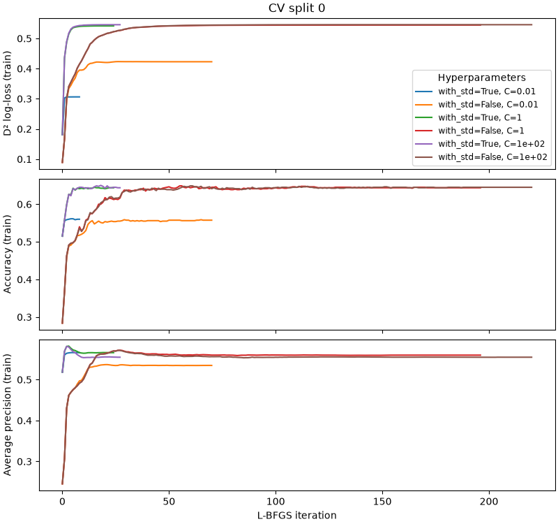
We define labels for plotting purposes and plot each metric separately.
cv_lbfgs_log["param_label"] = cv_lbfgs_log.apply(
    lambda row: (
        f"with_std={row['param_standardscaler__with_std']}, "
        f"C={row['param_logisticregression__C']:.2g}"
    ),
    axis=1,
)

metrics = {
    "d2_log_loss_score": "D² log-loss (train)",
    "accuracy": "Accuracy (train)",
    "average_precision": "Average precision (train)",
}
_, axes = plt.subplots(
    len(metrics),
    1,
    figsize=(8, 2.5 * len(metrics)),
    sharex=True,
    constrained_layout=True,
)
for idx, (metric, ylabel) in enumerate(metrics.items()):
    ax = axes[idx]
    for param_label, group in cv_lbfgs_log.groupby("param_label", sort=False):
        ax.plot(group["task_id"], group[metric], label=param_label)
    ax.set_ylabel(ylabel)
    if idx == 0:
        ax.set_title("CV split 0")
        ax.legend(title="Hyperparameters", fontsize="small")

_ = axes[-1].set_xlabel("L-BFGS iteration")
Analysis of the convergence of the logistic regression models#
D² log-loss convergence#
The D² log-loss scores generally improve monotonically for all models. This
is expected because the logistic regression model is fitted by minimizing the
(regularized) log-loss computed on the training set.
Accuracy fluctuations#
The accuracy score improves with the number of iterations, albeit with some
local fluctuations. This is expected because accuracy is discontinuous and
not directly optimized by the model. Instead the model minimizes the log-loss
which is a smooth surrogate for the zero-one loss (and thus related to, but
not directly optimized by, accuracy).
Regularization and scaling#
We also observe that the least regularized models (larger C values) tend
to reach higher D² log-loss scores, and models trained on scaled features
converge in much fewer iterations.
Furthermore, models trained with high regularization (lower C values)
converge to a final D² log-loss value that depends on the regularization
strength while this is not the case for models trained with low
regularization: there is a strong coupling between the optimal regularization
strength and the feature scaling.
Average precision vs log-loss, refinement vs calibration#
Finally, we observe that the average precision value measured on the training
set can improve quickly in the first iterations and then worsen even though
the D² log-loss value continues to improve on the same training data. This is
especially noticeable for models trained with low regularization and feature
standardization. This counter-intuitive behavior can be explained as follows.
First recall that average precision is a pure ranking metric that measures
the ability of the model to output predicted probabilities that rank the
samples of a given class higher than the samples of the other classes, but
does not take into account the calibration of the predicted probabilities. In
other words, average precision only evaluates if the predicted probabilities
are well ordered relatively to one another but is insensitive to a rank
preserving transformation of their absolute values. The log-loss, on the
other hand, is a strictly proper scoring rule that accounts for both the
refinement (ranking power) of the model and the calibration of the predicted
probabilities.
Therefore, the average precision curves of the low-regularized models trained
on scaled features suggest that the first iterations mostly improve
refinement of the models temporarily leaving calibration behind. In later
iterations, the log-loss score continues to improve but average precision
values worsen, which suggests that the logistic regression model
progressively trades off refinement for calibration over the course of the
final iterations. This phenomenon has been studied in [1].
It would be interesting to see if this also happens when evaluating the model
on a validation set so we could implement early stopping on average precision
to explicitly select a model with high refinement on a validation set. This
is not yet possible at the time of writing. Giving callbacks access to the
validation set is planned for a future version of scikit-learn. Note that the
callbacks API is still experimental and may change without the usual
deprecation cycle.
|