Note

Go to the end to download the full example code or to run this example in your browser via JupyterLite or Binder.

Visualizations with Display Objects#

In this example, we will construct display objects, ConfusionMatrixDisplay, RocCurveDisplay, and PrecisionRecallDisplay directly from their respective metrics. This is an alternative to using their corresponding plot functions when a model’s predictions are already computed or expensive to compute. Note that this is advanced usage, and in general we recommend using their respective plot functions.

# Authors: The scikit-learn developers
# SPDX-License-Identifier: BSD-3-Clause

Load Data and train model#

For this example, we load a blood transfusion service center data set from OpenML. This is a binary classification problem where the target is whether an individual donated blood. Then the data is split into a train and test dataset and a logistic regression is fitted with the train dataset.

from sklearn.datasets import fetch_openml
from sklearn.linear_model import LogisticRegression
from sklearn.model_selection import train_test_split
from sklearn.pipeline import make_pipeline
from sklearn.preprocessing import StandardScaler

X, y = fetch_openml(data_id=1464, return_X_y=True)
X_train, X_test, y_train, y_test = train_test_split(X, y, stratify=y)

clf = make_pipeline(StandardScaler(), LogisticRegression(random_state=0))
clf.fit(X_train, y_train)

Pipeline(steps=[('standardscaler', StandardScaler()),
                ('logisticregression', LogisticRegression(random_state=0))])

In a Jupyter environment, please rerun this cell to show the HTML representation or trust the notebook.
On GitHub, the HTML representation is unable to render, please try loading this page with nbviewer.org.

Pipeline

?Documentation for PipelineiFitted

Parameters

	steps steps: list of tuples List of (name of step, estimator) tuples that are to be chained in sequential order. To be compatible with the scikit-learn API, all steps must define `fit`. All non-last steps must also define `transform`. See :ref:`Combining Estimators <combining_estimators>` for more details.	[('standardscaler', ...), ('logisticregression', ...)]
	transform_input transform_input: list of str, default=None The names of the :term:`metadata` parameters that should be transformed by the pipeline before passing it to the step consuming it. This enables transforming some input arguments to ``fit`` (other than ``X``) to be transformed by the steps of the pipeline up to the step which requires them. Requirement is defined via :ref:`metadata routing <metadata_routing>`. For instance, this can be used to pass a validation set through the pipeline. You can only set this if metadata routing is enabled, which you can enable using ``sklearn.set_config(enable_metadata_routing=True)``. .. versionadded:: 1.6	None
	memory memory: str or object with the joblib.Memory interface, default=None Used to cache the fitted transformers of the pipeline. The last step will never be cached, even if it is a transformer. By default, no caching is performed. If a string is given, it is the path to the caching directory. Enabling caching triggers a clone of the transformers before fitting. Therefore, the transformer instance given to the pipeline cannot be inspected directly. Use the attribute ``named_steps`` or ``steps`` to inspect estimators within the pipeline. Caching the transformers is advantageous when fitting is time consuming. See :ref:`sphx_glr_auto_examples_neighbors_plot_caching_nearest_neighbors.py` for an example on how to enable caching.	None
	verbose verbose: bool, default=False If True, the time elapsed while fitting each step will be printed as it is completed.	False

Fitted attributes

Name	Type	Value
classes_ classes_: ndarray of shape (n_classes,) The classes labels. Only exist if the last step of the pipeline is a classifier.	ndarray[object](2,)	['1','2']
feature_names_in_ feature_names_in_: ndarray of shape (`n_features_in_`,) Names of features seen during :term:`fit`. Only defined if the underlying estimator exposes such an attribute when fit. .. versionadded:: 1.0	ndarray[object](4,)	['V1','V2','V3','V4']
n_features_in_ n_features_in_: int Number of features seen during :term:`fit`. Only defined if the underlying first estimator in `steps` exposes such an attribute when fit. .. versionadded:: 0.24	int	4

StandardScaler

?Documentation for StandardScaler

Parameters

	copy copy: bool, default=True If False, try to avoid a copy and do inplace scaling instead. This is not guaranteed to always work inplace; e.g. if the data is not a NumPy array or scipy.sparse CSR matrix, a copy may still be returned.	True
	with_mean with_mean: bool, default=True If True, center the data before scaling. This does not work (and will raise an exception) when attempted on sparse matrices, because centering them entails building a dense matrix which in common use cases is likely to be too large to fit in memory.	True
	with_std with_std: bool, default=True If True, scale the data to unit variance (or equivalently, unit standard deviation).	True

Fitted attributes

Name	Type	Value
feature_names_in_ feature_names_in_: ndarray of shape (`n_features_in_`,) Names of features seen during :term:`fit`. Defined only when `X` has feature names that are all strings. .. versionadded:: 1.0	ndarray[object](4,)	['V1','V2','V3','V4']
mean_ mean_: ndarray of shape (n_features,) or None The mean value for each feature in the training set. Equal to ``None`` when ``with_mean=False`` and ``with_std=False``.	ndarray[float64](4,)	[ 9.82, 5.32,1330.66, 34.18]
n_features_in_ n_features_in_: int Number of features seen during :term:`fit`. .. versionadded:: 0.24	int	4
n_samples_seen_ n_samples_seen_: int or ndarray of shape (n_features,) The number of samples processed by the estimator for each feature. If there are no missing samples, the ``n_samples_seen`` will be an integer, otherwise it will be an array of dtype int. If `sample_weights` are used it will be a float (if no missing data) or an array of dtype float that sums the weights seen so far. Will be reset on new calls to fit, but increments across ``partial_fit`` calls.	float64	561
scale_ scale_: ndarray of shape (n_features,) or None Per feature relative scaling of the data to achieve zero mean and unit variance. Generally this is calculated using `np.sqrt(var_)`. If a variance is zero, we can't achieve unit variance, and the data is left as-is, giving a scaling factor of 1. `scale_` is equal to `None` when `with_std=False`. .. versionadded:: 0.17 scale_	ndarray[float64](4,)	[ 8.3 , 5.34,1335.97, 23.33]
var_ var_: ndarray of shape (n_features,) or None The variance for each feature in the training set. Used to compute `scale_`. Equal to ``None`` when ``with_mean=False`` and ``with_std=False``.	ndarray[float64](4,)	[ 68.95, 28.56,1784826.48, 544.31]

4 features

LogisticRegression

?Documentation for LogisticRegression

Parameters

	random_state random_state: int, RandomState instance, default=None Only used for `solver` == 'sag', 'saga' or 'liblinear' to shuffle the data. It has no effect on the other solvers. See :term:`Glossary <random_state>` for details.	0
	penalty penalty: {'l1', 'l2', 'elasticnet', None}, default='l2' Specify the norm of the penalty: - `None`: no penalty is added; - `'l2'`: add an L2 penalty term and it is the default choice; - `'l1'`: add an L1 penalty term; - `'elasticnet'`: both L1 and L2 penalty terms are added. .. warning:: Some penalties may not work with some solvers. See the parameter `solver` below, to know the compatibility between the penalty and solver. .. versionadded:: 0.19 l1 penalty with SAGA solver (allowing 'multinomial' + L1) .. deprecated:: 1.8 `penalty` was deprecated in version 1.8 and will be removed in 1.10. Use `l1_ratio` and `C` instead. `l1_ratio=0` for `penalty='l2'`, `l1_ratio=1` for `penalty='l1'`, `l1_ratio` set to any float between 0 and 1 for `penalty='elasticnet'`, and `C=np.inf` for `penalty=None`.	'deprecated'
	C C: float, default=1.0 Inverse of regularization strength; must be a positive float. Like in support vector machines, smaller values specify stronger regularization. `C=np.inf` results in unpenalized logistic regression. For a visual example on the effect of tuning the `C` parameter with an L1 penalty, see: :ref:`sphx_glr_auto_examples_linear_model_plot_logistic_path.py`.	1.0
	l1_ratio l1_ratio: float, default=0.0 The Elastic-Net mixing parameter, with `0 <= l1_ratio <= 1`. Setting `l1_ratio=1` gives a pure L1-penalty, setting `l1_ratio=0` a pure L2-penalty. Any value between 0 and 1 gives an Elastic-Net penalty of the form `l1_ratio * L1 + (1 - l1_ratio) * L2`. .. warning:: Certain values of `l1_ratio`, i.e. some penalties, may not work with some solvers. See the parameter `solver` below, to know the compatibility between the penalty and solver. .. versionchanged:: 1.8 Default value changed from None to 0.0. .. deprecated:: 1.8 `None` is deprecated and will be removed in version 1.10. Always use `l1_ratio` to specify the penalty type.	0.0
	dual dual: bool, default=False Dual (constrained) or primal (regularized, see also :ref:`this equation <regularized-logistic-loss>`) formulation. Dual formulation is only implemented for l2 penalty with liblinear solver. Prefer `dual=False` when n_samples > n_features.	False
	tol tol: float, default=1e-4 Tolerance for stopping criteria.	0.0001
	fit_intercept fit_intercept: bool, default=True Specifies if a constant (a.k.a. bias or intercept) should be added to the decision function.	True
	intercept_scaling intercept_scaling: float, default=1 Useful only when the solver `liblinear` is used and `self.fit_intercept` is set to `True`. In this case, `x` becomes `[x, self.intercept_scaling]`, i.e. a "synthetic" feature with constant value equal to `intercept_scaling` is appended to the instance vector. The intercept becomes ``intercept_scaling * synthetic_feature_weight``. .. note:: The synthetic feature weight is subject to L1 or L2 regularization as all other features. To lessen the effect of regularization on synthetic feature weight (and therefore on the intercept) `intercept_scaling` has to be increased.	1
	class_weight class_weight: dict or 'balanced', default=None Weights associated with classes in the form ``{class_label: weight}``. If not given, all classes are supposed to have weight one. The "balanced" mode uses the values of y to automatically adjust weights inversely proportional to class frequencies in the input data as ``n_samples / (n_classes * np.bincount(y))``. Note that these weights will be multiplied with sample_weight (passed through the fit method) if sample_weight is specified. .. versionadded:: 0.17 class_weight='balanced'	None
	solver solver: {'lbfgs', 'liblinear', 'newton-cg', 'newton-cholesky', 'sag', 'saga'}, default='lbfgs' Algorithm to use in the optimization problem. Default is 'lbfgs'. To choose a solver, you might want to consider the following aspects: - 'lbfgs' is a good default solver because it works reasonably well for a wide class of problems. - For :term:`multiclass` problems (`n_classes >= 3`), all solvers except 'liblinear' minimize the full multinomial loss, 'liblinear' will raise an error. - 'newton-cholesky' is a good choice for `n_samples` >> `n_features * n_classes`, especially with one-hot encoded categorical features with rare categories. Be aware that the memory usage of this solver has a quadratic dependency on `n_features * n_classes` because it explicitly computes the full Hessian matrix. - For small datasets, 'liblinear' is a good choice, whereas 'sag' and 'saga' are faster for large ones; - 'liblinear' can only handle binary classification by default. To apply a one-versus-rest scheme for the multiclass setting one can wrap it with the :class:`~sklearn.multiclass.OneVsRestClassifier`. .. warning:: The choice of the algorithm depends on the penalty chosen (`l1_ratio=0` for L2-penalty, `l1_ratio=1` for L1-penalty and `0 < l1_ratio < 1` for Elastic-Net) and on (multinomial) multiclass support: ================= ======================== ====================== solver l1_ratio multinomial multiclass ================= ======================== ====================== 'lbfgs' l1_ratio=0 yes 'liblinear' l1_ratio=1 or l1_ratio=0 no 'newton-cg' l1_ratio=0 yes 'newton-cholesky' l1_ratio=0 yes 'sag' l1_ratio=0 yes 'saga' 0<=l1_ratio<=1 yes ================= ======================== ====================== .. note:: 'sag' and 'saga' fast convergence is only guaranteed on features with approximately the same scale. You can preprocess the data with a scaler from :mod:`sklearn.preprocessing`. .. seealso:: Refer to the :ref:`User Guide <Logistic_regression>` for more information regarding :class:`LogisticRegression` and more specifically the :ref:`Table <logistic_regression_solvers>` summarizing solver/penalty supports. .. versionadded:: 0.17 Stochastic Average Gradient (SAG) descent solver. Multinomial support in version 0.18. .. versionadded:: 0.19 SAGA solver. .. versionchanged:: 0.22 The default solver changed from 'liblinear' to 'lbfgs' in 0.22. .. versionadded:: 1.2 newton-cholesky solver. Multinomial support in version 1.6.	'lbfgs'
	max_iter max_iter: int, default=100 Maximum number of iterations taken for the solvers to converge.	100
	verbose verbose: int, default=0 For the liblinear and lbfgs solvers set verbose to any positive number for verbosity.	0
	warm_start warm_start: bool, default=False When set to True, reuse the solution of the previous call to fit as initialization, otherwise, just erase the previous solution. Useless for liblinear solver. See :term:`the Glossary <warm_start>`. .. versionadded:: 0.17 warm_start to support lbfgs, newton-cg, sag, saga solvers.	False
	n_jobs n_jobs: int, default=None Does not have any effect. .. deprecated:: 1.8 `n_jobs` is deprecated in version 1.8 and will be removed in 1.10.	None

Fitted attributes

Name	Type	Value
classes_ classes_: ndarray of shape (n_classes, ) A list of class labels known to the classifier.	ndarray[object](2,)	['1','2']
coef_ coef_: ndarray or CSR matrix of shape (1, n_features) or (n_classes, n_features) Coefficients of the features in the decision function. `coef_` is of shape (1, n_features) when the given problem is binary. By default, it will be created as a dense array, but can be turned to sparse (CSR format) through :meth:`sparsify` (which can be beneficial under L1 regularization when many coefficients are zero), and back to dense through :meth:`densify`.	ndarray[float64](1, 4)	[[-0.74, 0.38, 0.38,-0.53]]
intercept_ intercept_: ndarray of shape (1,) or (n_classes,) Intercept (a.k.a. bias) added to the decision function. If `fit_intercept` is set to False, the intercept is set to zero. `intercept_` is of shape (1,) when the given problem is binary.	ndarray[float64](1,)	[-1.41]
n_features_in_ n_features_in_: int Number of features seen during :term:`fit`. .. versionadded:: 0.24	int	4
n_iter_ n_iter_: ndarray of shape (1, ) Actual number of iterations for all classes. .. versionchanged:: 0.20 In SciPy <= 1.0.0 the number of lbfgs iterations may exceed ``max_iter``. ``n_iter_`` will now report at most ``max_iter``.	ndarray[int32](1,)	[8]

Create `ConfusionMatrixDisplay`#

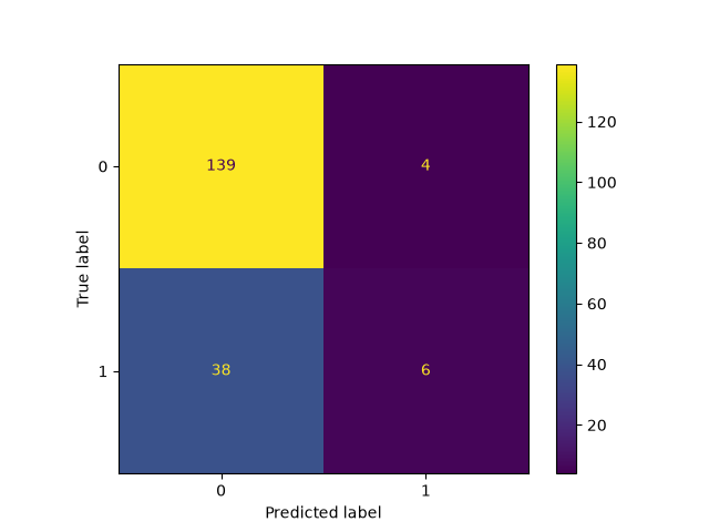
With the fitted model, we compute the predictions of the model on the test dataset. These predictions are used to compute the confusion matrix which is plotted with the ConfusionMatrixDisplay

from sklearn.metrics import ConfusionMatrixDisplay, confusion_matrix

y_pred = clf.predict(X_test)
cm = confusion_matrix(y_test, y_pred)

cm_display = ConfusionMatrixDisplay(cm).plot()

Create `RocCurveDisplay`#

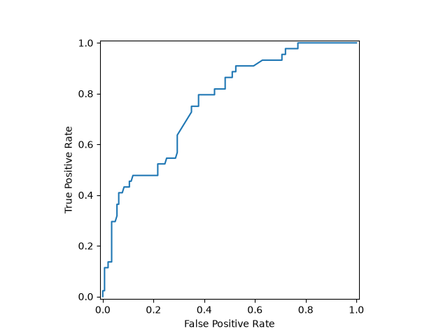
The roc curve requires either the probabilities or the non-thresholded decision values from the estimator. Since the logistic regression provides a decision function, we will use it to plot the roc curve:

from sklearn.metrics import RocCurveDisplay, roc_curve

y_score = clf.decision_function(X_test)

fpr, tpr, _ = roc_curve(y_test, y_score, pos_label=clf.classes_[1])
roc_display = RocCurveDisplay(fpr=fpr, tpr=tpr).plot()

Create `PrecisionRecallDisplay`#

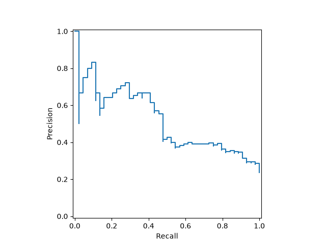
Similarly, the precision recall curve can be plotted using y_score from the prevision sections.

from sklearn.metrics import PrecisionRecallDisplay, precision_recall_curve

prec, recall, _ = precision_recall_curve(y_test, y_score, pos_label=clf.classes_[1])
pr_display = PrecisionRecallDisplay(precision=prec, recall=recall).plot()

Combining the display objects into a single plot#

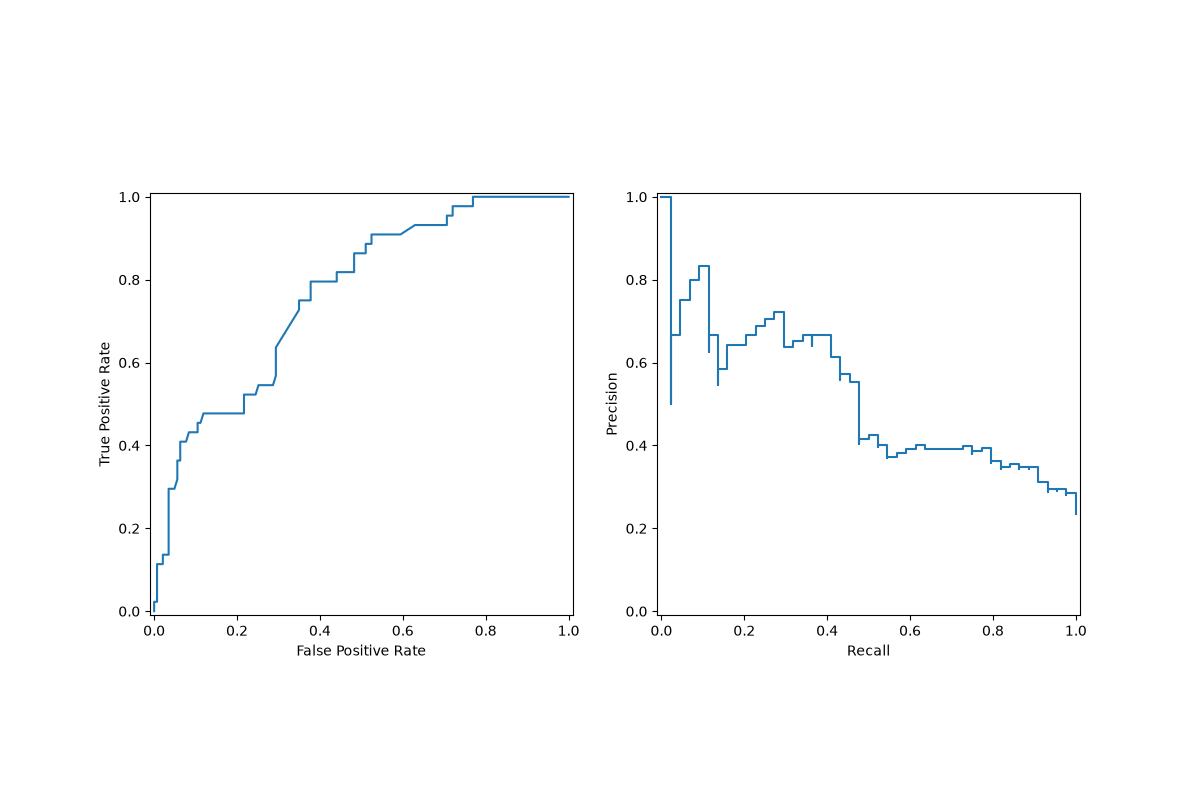
The display objects store the computed values that were passed as arguments. This allows for the visualizations to be easily combined using matplotlib’s API. In the following example, we place the displays next to each other in a row.

import matplotlib.pyplot as plt

fig, (ax1, ax2) = plt.subplots(1, 2, figsize=(12, 8))

roc_display.plot(ax=ax1)
pr_display.plot(ax=ax2)
plt.show()

Total running time of the script: (0 minutes 0.308 seconds)

Download Jupyter notebook: plot_display_object_visualization.ipynb

Download Python source code: plot_display_object_visualization.py

Download zipped: plot_display_object_visualization.zip

Related examples

Precision-Recall

ROC Curve with Visualization API

Multiclass Receiver Operating Characteristic (ROC)

Post-tuning the decision threshold for cost-sensitive learning

Gallery generated by Sphinx-Gallery

GeezerVison

Visualizations with Display Objects#

Load Data and train model#

Create ConfusionMatrixDisplay#

Create RocCurveDisplay#

Create PrecisionRecallDisplay#

Combining the display objects into a single plot#

Create `ConfusionMatrixDisplay`#

Create `RocCurveDisplay`#

Create `PrecisionRecallDisplay`#