Note

Go to the end to download the full example code or to run this example in your browser via JupyterLite or Binder.

Probability Calibration for 3-class classification#

This example illustrates how sigmoid calibration changes predicted probabilities for a 3-class classification problem. Illustrated is the standard 2-simplex, where the three corners correspond to the three classes. Arrows point from the probability vectors predicted by an uncalibrated classifier to the probability vectors predicted by the same classifier after sigmoid calibration on a hold-out validation set. Colors indicate the true class of an instance (red: class 1, green: class 2, blue: class 3).

Data#

Below, we generate a classification dataset with 2000 samples, 2 features and 3 target classes. We then split the data as follows:

train: 600 samples (for training the classifier)
valid: 400 samples (for calibrating predicted probabilities)
test: 1000 samples

Note that we also create X_train_valid and y_train_valid, which consists of both the train and valid subsets. This is used when we only want to train the classifier but not calibrate the predicted probabilities.

# Authors: The scikit-learn developers
# SPDX-License-Identifier: BSD-3-Clause

import numpy as np

from sklearn.datasets import make_blobs

np.random.seed(0)

X, y = make_blobs(
    n_samples=2000, n_features=2, centers=3, random_state=42, cluster_std=5.0
)
X_train, y_train = X[:600], y[:600]
X_valid, y_valid = X[600:1000], y[600:1000]
X_train_valid, y_train_valid = X[:1000], y[:1000]
X_test, y_test = X[1000:], y[1000:]

Fitting and calibration#

First, we will train a RandomForestClassifier with 25 base estimators (trees) on the concatenated train and validation data (1000 samples). This is the uncalibrated classifier.

from sklearn.ensemble import RandomForestClassifier

clf = RandomForestClassifier(n_estimators=25)
clf.fit(X_train_valid, y_train_valid)

RandomForestClassifier(n_estimators=25)

In a Jupyter environment, please rerun this cell to show the HTML representation or trust the notebook.
On GitHub, the HTML representation is unable to render, please try loading this page with nbviewer.org.

RandomForestClassifier

?Documentation for RandomForestClassifieriFitted

Parameters

	n_estimators n_estimators: int, default=100 The number of trees in the forest. .. versionchanged:: 0.22 The default value of ``n_estimators`` changed from 10 to 100 in 0.22.	25
	criterion criterion: {"gini", "entropy", "log_loss"}, default="gini" The function to measure the quality of a split. Supported criteria are "gini" for the Gini impurity and "log_loss" and "entropy" both for the Shannon information gain, see :ref:`tree_mathematical_formulation`. Note: This parameter is tree-specific.	'gini'
	max_depth max_depth: int, default=None The maximum depth of the tree. If None, then nodes are expanded until all leaves are pure or until all leaves contain less than min_samples_split samples.	None
	min_samples_split min_samples_split: int or float, default=2 The minimum number of samples required to split an internal node: - If int, then consider `min_samples_split` as the minimum number. - If float, then `min_samples_split` is a fraction and `ceil(min_samples_split * n_samples)` are the minimum number of samples for each split. .. versionchanged:: 0.18 Added float values for fractions.	2
	min_samples_leaf min_samples_leaf: int or float, default=1 The minimum number of samples required to be at a leaf node. A split point at any depth will only be considered if it leaves at least ``min_samples_leaf`` training samples in each of the left and right branches. This may have the effect of smoothing the model, especially in regression. - If int, then consider `min_samples_leaf` as the minimum number. - If float, then `min_samples_leaf` is a fraction and `ceil(min_samples_leaf * n_samples)` are the minimum number of samples for each node. .. versionchanged:: 0.18 Added float values for fractions.	1
	min_weight_fraction_leaf min_weight_fraction_leaf: float, default=0.0 The minimum weighted fraction of the sum total of weights (of all the input samples) required to be at a leaf node. Samples have equal weight when sample_weight is not provided.	0.0
	max_features max_features: {"sqrt", "log2", None}, int or float, default="sqrt" The number of features to consider when looking for the best split: - If int, then consider `max_features` features at each split. - If float, then `max_features` is a fraction and `max(1, int(max_features * n_features_in_))` features are considered at each split. - If "sqrt", then `max_features=sqrt(n_features)`. - If "log2", then `max_features=log2(n_features)`. - If None, then `max_features=n_features`. .. versionchanged:: 1.1 The default of `max_features` changed from `"auto"` to `"sqrt"`. Note: the search for a split does not stop until at least one valid partition of the node samples is found, even if it requires to effectively inspect more than ``max_features`` features.	'sqrt'
	max_leaf_nodes max_leaf_nodes: int, default=None Grow trees with ``max_leaf_nodes`` in best-first fashion. Best nodes are defined as relative reduction in impurity. If None then unlimited number of leaf nodes.	None
	min_impurity_decrease min_impurity_decrease: float, default=0.0 A node will be split if this split induces a decrease of the impurity greater than or equal to this value. The weighted impurity decrease equation is the following:: N_t / N * (impurity - N_t_R / N_t * right_impurity - N_t_L / N_t * left_impurity) where ``N`` is the total number of samples, ``N_t`` is the number of samples at the current node, ``N_t_L`` is the number of samples in the left child, and ``N_t_R`` is the number of samples in the right child. ``N``, ``N_t``, ``N_t_R`` and ``N_t_L`` all refer to the weighted sum, if ``sample_weight`` is passed. .. versionadded:: 0.19	0.0
	bootstrap bootstrap: bool, default=True Whether bootstrap samples are used when building trees. If False, the whole dataset is used to build each tree.	True
	oob_score oob_score: bool or callable, default=False Whether to use out-of-bag samples to estimate the generalization score. By default, :func:`~sklearn.metrics.accuracy_score` is used. Provide a callable with signature `metric(y_true, y_pred)` to use a custom metric. Only available if `bootstrap=True`. For an illustration of out-of-bag (OOB) error estimation, see the example :ref:`sphx_glr_auto_examples_ensemble_plot_ensemble_oob.py`.	False
	n_jobs n_jobs: int, default=None The number of jobs to run in parallel. :meth:`fit`, :meth:`predict`, :meth:`decision_path` and :meth:`apply` are all parallelized over the trees. ``None`` means 1 unless in a :obj:`joblib.parallel_backend` context. ``-1`` means using all processors. See :term:`Glossary <n_jobs>` for more details.	None
	random_state random_state: int, RandomState instance or None, default=None Controls both the randomness of the bootstrapping of the samples used when building trees (if ``bootstrap=True``) and the sampling of the features to consider when looking for the best split at each node (if ``max_features < n_features``). See :term:`Glossary <random_state>` for details.	None
	verbose verbose: int, default=0 Controls the verbosity when fitting and predicting.	0
	warm_start warm_start: bool, default=False When set to ``True``, reuse the solution of the previous call to fit and add more estimators to the ensemble, otherwise, just fit a whole new forest. See :term:`Glossary <warm_start>` and :ref:`tree_ensemble_warm_start` for details.	False
	class_weight class_weight: {"balanced", "balanced_subsample"}, dict or list of dicts, default=None Weights associated with classes in the form ``{class_label: weight}``. If not given, all classes are supposed to have weight one. For multi-output problems, a list of dicts can be provided in the same order as the columns of y. Note that for multioutput (including multilabel) weights should be defined for each class of every column in its own dict. For example, for four-class multilabel classification weights should be [{0: 1, 1: 1}, {0: 1, 1: 5}, {0: 1, 1: 1}, {0: 1, 1: 1}] instead of [{1:1}, {2:5}, {3:1}, {4:1}]. The "balanced" mode uses the values of y to automatically adjust weights inversely proportional to class frequencies in the input data as ``n_samples / (n_classes * np.bincount(y))`` The "balanced_subsample" mode is the same as "balanced" except that weights are computed based on the bootstrap sample for every tree grown. For multi-output, the weights of each column of y will be multiplied. Note that these weights will be multiplied with sample_weight (passed through the fit method) if sample_weight is specified.	None
	ccp_alpha ccp_alpha: non-negative float, default=0.0 Complexity parameter used for Minimal Cost-Complexity Pruning. The subtree with the largest cost complexity that is smaller than ``ccp_alpha`` will be chosen. By default, no pruning is performed. See :ref:`minimal_cost_complexity_pruning` for details. See :ref:`sphx_glr_auto_examples_tree_plot_cost_complexity_pruning.py` for an example of such pruning. .. versionadded:: 0.22	0.0
	max_samples max_samples: int or float, default=None If bootstrap is True, the number of samples to draw from X to train each base estimator. - If None (default), then draw `X.shape[0]` samples irrespective of `sample_weight`. - If int, then draw `max_samples` samples. - If float, then draw `max_samples * X.shape[0]` unweighted samples or `max_samples * sample_weight.sum()` weighted samples. .. versionadded:: 0.22 .. versionchanged:: 1.9 Float `max_samples` is relative to `sample_weight.sum()` instead of `X.shape[0]` for weighted samples.	None
	monotonic_cst monotonic_cst: array-like of int of shape (n_features,), default=None Indicates the monotonicity constraint to enforce on each feature. - 1: monotonically increasing - 0: no constraint - -1: monotonically decreasing If monotonic_cst is None, no constraints are applied. Monotonicity constraints are not supported for: - multiclass classifications (i.e. when `n_classes > 2`), - multioutput classifications (i.e. when `n_outputs_ > 1`). The constraints hold over the probability of the positive class. Read more in the :ref:`User Guide <monotonic_cst_gbdt>`. .. versionadded:: 1.4	None

Fitted attributes

Name	Type	Value
classes_ classes_: ndarray of shape (n_classes,) or a list of such arrays The classes labels (single output problem), or a list of arrays of class labels (multi-output problem).	ndarray[int64](3,)	[0,1,2]
estimator_ estimator_: :class:`~sklearn.tree.DecisionTreeClassifier` The child estimator template used to create the collection of fitted sub-estimators. .. versionadded:: 1.2 `base_estimator_` was renamed to `estimator_`.	DecisionTreeClassifier	DecisionTreeClassifier()
estimators_ estimators_: list of DecisionTreeClassifier The collection of fitted sub-estimators.	list	[DecisionTreeC...ate=209652396), DecisionTreeC...ate=398764591), DecisionTreeC...ate=924231285), DecisionTreeC...te=1478610112), ...]
estimators_samples_ estimators_samples_: list of arrays The subset of drawn samples (i.e., the in-bag samples) for each base estimator. Each subset is defined by an array of the indices selected. .. versionadded:: 1.4	list	[array([236, 2... dtype=int32), array([107, 1... dtype=int32), array([301, 5... dtype=int32), array([900, 3... dtype=int32), ...]
feature_importances_ feature_importances_: ndarray of shape (n_features,) The impurity-based feature importances. The higher, the more important the feature. The importance of a feature is computed as the (normalized) total reduction of the criterion brought by that feature. It is also known as the Gini importance. Warning: impurity-based feature importances can be misleading for high cardinality features (many unique values). See :func:`sklearn.inspection.permutation_importance` as an alternative.	ndarray[float64](2,)	[0.44,0.56]
n_classes_ n_classes_: int or list The number of classes (single output problem), or a list containing the number of classes for each output (multi-output problem).	int	3
n_features_in_ n_features_in_: int Number of features seen during :term:`fit`. .. versionadded:: 0.24	int	2
n_outputs_ n_outputs_: int The number of outputs when ``fit`` is performed.	int	1

To train the calibrated classifier, we start with the same RandomForestClassifier but train it using only the train data subset (600 samples) then calibrate, with method='sigmoid', using the valid data subset (400 samples) in a 2-stage process.

from sklearn.calibration import CalibratedClassifierCV
from sklearn.frozen import FrozenEstimator

clf = RandomForestClassifier(n_estimators=25)
clf.fit(X_train, y_train)
cal_clf = CalibratedClassifierCV(FrozenEstimator(clf), method="sigmoid")
cal_clf.fit(X_valid, y_valid)

CalibratedClassifierCV(estimator=FrozenEstimator(estimator=RandomForestClassifier(n_estimators=25)))

CalibratedClassifierCV

?Documentation for CalibratedClassifierCViFitted

Parameters

	estimator estimator: estimator instance, default=None The classifier whose output need to be calibrated to provide more accurate `predict_proba` outputs. The default classifier is a :class:`~sklearn.svm.LinearSVC`. .. versionadded:: 1.2	FrozenEstimat...stimators=25))
	method method: {'sigmoid', 'isotonic', 'temperature'}, default='sigmoid' The method to use for calibration. Can be: - 'sigmoid', which corresponds to Platt's method (i.e. a binary logistic regression model). - 'isotonic', which is a non-parametric approach. - 'temperature', temperature scaling. Sigmoid and isotonic calibration methods natively support only binary classifiers and extend to multi-class classification using a One-vs-Rest (OvR) strategy with post-hoc renormalization, i.e., adjusting the probabilities after calibration to ensure they sum up to 1. In contrast, temperature scaling naturally supports multi-class calibration by applying `softmax(classifier_logits/T)` with a value of `T` (temperature) that optimizes the log loss. For very uncalibrated classifiers on very imbalanced datasets, sigmoid calibration might be preferred because it fits an additional intercept parameter. This helps shift decision boundaries appropriately when the classifier being calibrated is biased towards the majority class. Isotonic calibration is not recommended when the number of calibration samples is too low ``(≪1000)`` since it then tends to overfit. .. versionchanged:: 1.8 Added option 'temperature'.	'sigmoid'
	cv cv: int, cross-validation generator, or iterable, default=None Determines the cross-validation splitting strategy. Possible inputs for cv are: - None, to use the default 5-fold cross-validation, - integer, to specify the number of folds, - :term:`CV splitter`, - an iterable yielding (train, test) splits as arrays of indices. For integer/None inputs, if ``y`` is binary or multiclass, :class:`~sklearn.model_selection.StratifiedKFold` is used. If ``y`` is neither binary nor multiclass, :class:`~sklearn.model_selection.KFold` is used. Refer to the :ref:`User Guide <cross_validation>` for the various cross-validation strategies that can be used here. .. versionchanged:: 0.22 ``cv`` default value if None changed from 3-fold to 5-fold.	None
	n_jobs n_jobs: int, default=None Number of jobs to run in parallel. ``None`` means 1 unless in a :obj:`joblib.parallel_backend` context. ``-1`` means using all processors. Base estimator clones are fitted in parallel across cross-validation iterations. See :term:`Glossary <n_jobs>` for more details. .. versionadded:: 0.24	None
	ensemble ensemble: bool, or "auto", default="auto" Determines how the calibrator is fitted. "auto" will use `False` if the `estimator` is a :class:`~sklearn.frozen.FrozenEstimator`, and `True` otherwise. If `True`, the `estimator` is fitted using training data, and calibrated using testing data, for each `cv` fold. The final estimator is an ensemble of `n_cv` fitted classifier and calibrator pairs, where `n_cv` is the number of cross-validation folds. The output is the average predicted probabilities of all pairs. If `False`, `cv` is used to compute unbiased predictions, via :func:`~sklearn.model_selection.cross_val_predict`, which are then used for calibration. At prediction time, the classifier used is the `estimator` trained on all the data. Note that this method is also internally implemented in :mod:`sklearn.svm` estimators with the `probabilities=True` parameter. .. versionadded:: 0.24 .. versionchanged:: 1.6 `"auto"` option is added and is the default.	'auto'

Fitted attributes

Name	Type	Value
calibrated_classifiers_ calibrated_classifiers_: list (len() equal to cv or 1 if `ensemble=False`) The list of classifier and calibrator pairs. - When `ensemble=True`, `n_cv` fitted `estimator` and calibrator pairs. `n_cv` is the number of cross-validation folds. - When `ensemble=False`, the `estimator`, fitted on all the data, and fitted calibrator. .. versionchanged:: 0.24 Single calibrated classifier case when `ensemble=False`.	list	[<sklearn.cali...x7e1dcbfc47e0>]
classes_ classes_: ndarray of shape (n_classes,) The class labels.	ndarray[int64](3,)	[0,1,2]
n_features_in_ n_features_in_: int Number of features seen during :term:`fit`. Only defined if the underlying estimator exposes such an attribute when fit. .. versionadded:: 0.24	int	2

estimator: FrozenEstimator

FrozenEstimator(estimator=RandomForestClassifier(n_estimators=25))

estimator: RandomForestClassifier

RandomForestClassifier(n_estimators=25)

RandomForestClassifier

?Documentation for RandomForestClassifier

Parameters

	n_estimators n_estimators: int, default=100 The number of trees in the forest. .. versionchanged:: 0.22 The default value of ``n_estimators`` changed from 10 to 100 in 0.22.	25
	criterion criterion: {"gini", "entropy", "log_loss"}, default="gini" The function to measure the quality of a split. Supported criteria are "gini" for the Gini impurity and "log_loss" and "entropy" both for the Shannon information gain, see :ref:`tree_mathematical_formulation`. Note: This parameter is tree-specific.	'gini'
	max_depth max_depth: int, default=None The maximum depth of the tree. If None, then nodes are expanded until all leaves are pure or until all leaves contain less than min_samples_split samples.	None
	min_samples_split min_samples_split: int or float, default=2 The minimum number of samples required to split an internal node: - If int, then consider `min_samples_split` as the minimum number. - If float, then `min_samples_split` is a fraction and `ceil(min_samples_split * n_samples)` are the minimum number of samples for each split. .. versionchanged:: 0.18 Added float values for fractions.	2
	min_samples_leaf min_samples_leaf: int or float, default=1 The minimum number of samples required to be at a leaf node. A split point at any depth will only be considered if it leaves at least ``min_samples_leaf`` training samples in each of the left and right branches. This may have the effect of smoothing the model, especially in regression. - If int, then consider `min_samples_leaf` as the minimum number. - If float, then `min_samples_leaf` is a fraction and `ceil(min_samples_leaf * n_samples)` are the minimum number of samples for each node. .. versionchanged:: 0.18 Added float values for fractions.	1
	min_weight_fraction_leaf min_weight_fraction_leaf: float, default=0.0 The minimum weighted fraction of the sum total of weights (of all the input samples) required to be at a leaf node. Samples have equal weight when sample_weight is not provided.	0.0
	max_features max_features: {"sqrt", "log2", None}, int or float, default="sqrt" The number of features to consider when looking for the best split: - If int, then consider `max_features` features at each split. - If float, then `max_features` is a fraction and `max(1, int(max_features * n_features_in_))` features are considered at each split. - If "sqrt", then `max_features=sqrt(n_features)`. - If "log2", then `max_features=log2(n_features)`. - If None, then `max_features=n_features`. .. versionchanged:: 1.1 The default of `max_features` changed from `"auto"` to `"sqrt"`. Note: the search for a split does not stop until at least one valid partition of the node samples is found, even if it requires to effectively inspect more than ``max_features`` features.	'sqrt'
	max_leaf_nodes max_leaf_nodes: int, default=None Grow trees with ``max_leaf_nodes`` in best-first fashion. Best nodes are defined as relative reduction in impurity. If None then unlimited number of leaf nodes.	None
	min_impurity_decrease min_impurity_decrease: float, default=0.0 A node will be split if this split induces a decrease of the impurity greater than or equal to this value. The weighted impurity decrease equation is the following:: N_t / N * (impurity - N_t_R / N_t * right_impurity - N_t_L / N_t * left_impurity) where ``N`` is the total number of samples, ``N_t`` is the number of samples at the current node, ``N_t_L`` is the number of samples in the left child, and ``N_t_R`` is the number of samples in the right child. ``N``, ``N_t``, ``N_t_R`` and ``N_t_L`` all refer to the weighted sum, if ``sample_weight`` is passed. .. versionadded:: 0.19	0.0
	bootstrap bootstrap: bool, default=True Whether bootstrap samples are used when building trees. If False, the whole dataset is used to build each tree.	True
	oob_score oob_score: bool or callable, default=False Whether to use out-of-bag samples to estimate the generalization score. By default, :func:`~sklearn.metrics.accuracy_score` is used. Provide a callable with signature `metric(y_true, y_pred)` to use a custom metric. Only available if `bootstrap=True`. For an illustration of out-of-bag (OOB) error estimation, see the example :ref:`sphx_glr_auto_examples_ensemble_plot_ensemble_oob.py`.	False
	n_jobs n_jobs: int, default=None The number of jobs to run in parallel. :meth:`fit`, :meth:`predict`, :meth:`decision_path` and :meth:`apply` are all parallelized over the trees. ``None`` means 1 unless in a :obj:`joblib.parallel_backend` context. ``-1`` means using all processors. See :term:`Glossary <n_jobs>` for more details.	None
	random_state random_state: int, RandomState instance or None, default=None Controls both the randomness of the bootstrapping of the samples used when building trees (if ``bootstrap=True``) and the sampling of the features to consider when looking for the best split at each node (if ``max_features < n_features``). See :term:`Glossary <random_state>` for details.	None
	verbose verbose: int, default=0 Controls the verbosity when fitting and predicting.	0
	warm_start warm_start: bool, default=False When set to ``True``, reuse the solution of the previous call to fit and add more estimators to the ensemble, otherwise, just fit a whole new forest. See :term:`Glossary <warm_start>` and :ref:`tree_ensemble_warm_start` for details.	False
	class_weight class_weight: {"balanced", "balanced_subsample"}, dict or list of dicts, default=None Weights associated with classes in the form ``{class_label: weight}``. If not given, all classes are supposed to have weight one. For multi-output problems, a list of dicts can be provided in the same order as the columns of y. Note that for multioutput (including multilabel) weights should be defined for each class of every column in its own dict. For example, for four-class multilabel classification weights should be [{0: 1, 1: 1}, {0: 1, 1: 5}, {0: 1, 1: 1}, {0: 1, 1: 1}] instead of [{1:1}, {2:5}, {3:1}, {4:1}]. The "balanced" mode uses the values of y to automatically adjust weights inversely proportional to class frequencies in the input data as ``n_samples / (n_classes * np.bincount(y))`` The "balanced_subsample" mode is the same as "balanced" except that weights are computed based on the bootstrap sample for every tree grown. For multi-output, the weights of each column of y will be multiplied. Note that these weights will be multiplied with sample_weight (passed through the fit method) if sample_weight is specified.	None
	ccp_alpha ccp_alpha: non-negative float, default=0.0 Complexity parameter used for Minimal Cost-Complexity Pruning. The subtree with the largest cost complexity that is smaller than ``ccp_alpha`` will be chosen. By default, no pruning is performed. See :ref:`minimal_cost_complexity_pruning` for details. See :ref:`sphx_glr_auto_examples_tree_plot_cost_complexity_pruning.py` for an example of such pruning. .. versionadded:: 0.22	0.0
	max_samples max_samples: int or float, default=None If bootstrap is True, the number of samples to draw from X to train each base estimator. - If None (default), then draw `X.shape[0]` samples irrespective of `sample_weight`. - If int, then draw `max_samples` samples. - If float, then draw `max_samples * X.shape[0]` unweighted samples or `max_samples * sample_weight.sum()` weighted samples. .. versionadded:: 0.22 .. versionchanged:: 1.9 Float `max_samples` is relative to `sample_weight.sum()` instead of `X.shape[0]` for weighted samples.	None
	monotonic_cst monotonic_cst: array-like of int of shape (n_features,), default=None Indicates the monotonicity constraint to enforce on each feature. - 1: monotonically increasing - 0: no constraint - -1: monotonically decreasing If monotonic_cst is None, no constraints are applied. Monotonicity constraints are not supported for: - multiclass classifications (i.e. when `n_classes > 2`), - multioutput classifications (i.e. when `n_outputs_ > 1`). The constraints hold over the probability of the positive class. Read more in the :ref:`User Guide <monotonic_cst_gbdt>`. .. versionadded:: 1.4	None

Fitted attributes

Name	Type	Value
classes_ classes_: ndarray of shape (n_classes,) or a list of such arrays The classes labels (single output problem), or a list of arrays of class labels (multi-output problem).	ndarray[int64](3,)	[0,1,2]
estimator_ estimator_: :class:`~sklearn.tree.DecisionTreeClassifier` The child estimator template used to create the collection of fitted sub-estimators. .. versionadded:: 1.2 `base_estimator_` was renamed to `estimator_`.	DecisionTreeClassifier	DecisionTreeClassifier()
estimators_ estimators_: list of DecisionTreeClassifier The collection of fitted sub-estimators.	list	[DecisionTreeC...te=1686997841), DecisionTreeC...te=1827923621), DecisionTreeC...te=1443447321), DecisionTreeC...ate=305097549), ...]
estimators_samples_ estimators_samples_: list of arrays The subset of drawn samples (i.e., the in-bag samples) for each base estimator. Each subset is defined by an array of the indices selected. .. versionadded:: 1.4	list	[array([ 66, ..., dtype=int32), array([313, 4..., dtype=int32), array([237, 4..., dtype=int32), array([ 1, 2..., dtype=int32), ...]
feature_importances_ feature_importances_: ndarray of shape (n_features,) The impurity-based feature importances. The higher, the more important the feature. The importance of a feature is computed as the (normalized) total reduction of the criterion brought by that feature. It is also known as the Gini importance. Warning: impurity-based feature importances can be misleading for high cardinality features (many unique values). See :func:`sklearn.inspection.permutation_importance` as an alternative.	ndarray[float64](2,)	[0.45,0.55]
n_classes_ n_classes_: int or list The number of classes (single output problem), or a list containing the number of classes for each output (multi-output problem).	int	3
n_features_in_ n_features_in_: int Number of features seen during :term:`fit`. .. versionadded:: 0.24	int	2
n_outputs_ n_outputs_: int The number of outputs when ``fit`` is performed.	int	1

Compare probabilities#

Below we plot a 2-simplex with arrows showing the change in predicted probabilities of the test samples.

import matplotlib.pyplot as plt

plt.figure(figsize=(10, 10))
colors = ["r", "g", "b"]

clf_probs = clf.predict_proba(X_test)
cal_clf_probs = cal_clf.predict_proba(X_test)
# Plot arrows
for i in range(clf_probs.shape[0]):
    plt.arrow(
        clf_probs[i, 0],
        clf_probs[i, 1],
        cal_clf_probs[i, 0] - clf_probs[i, 0],
        cal_clf_probs[i, 1] - clf_probs[i, 1],
        color=colors[y_test[i]],
        head_width=1e-2,
    )

# Plot perfect predictions, at each vertex
plt.plot([1.0], [0.0], "ro", ms=20, label="Class 1")
plt.plot([0.0], [1.0], "go", ms=20, label="Class 2")
plt.plot([0.0], [0.0], "bo", ms=20, label="Class 3")

# Plot boundaries of unit simplex
plt.plot([0.0, 1.0, 0.0, 0.0], [0.0, 0.0, 1.0, 0.0], "k", label="Simplex")

# Annotate points 6 points around the simplex, and mid point inside simplex
plt.annotate(
    r"($\frac{1}{3}$, $\frac{1}{3}$, $\frac{1}{3}$)",
    xy=(1.0 / 3, 1.0 / 3),
    xytext=(1.0 / 3, 0.23),
    xycoords="data",
    arrowprops=dict(facecolor="black", shrink=0.05),
    horizontalalignment="center",
    verticalalignment="center",
)
plt.plot([1.0 / 3], [1.0 / 3], "ko", ms=5)
plt.annotate(
    r"($\frac{1}{2}$, $0$, $\frac{1}{2}$)",
    xy=(0.5, 0.0),
    xytext=(0.5, 0.1),
    xycoords="data",
    arrowprops=dict(facecolor="black", shrink=0.05),
    horizontalalignment="center",
    verticalalignment="center",
)
plt.annotate(
    r"($0$, $\frac{1}{2}$, $\frac{1}{2}$)",
    xy=(0.0, 0.5),
    xytext=(0.1, 0.5),
    xycoords="data",
    arrowprops=dict(facecolor="black", shrink=0.05),
    horizontalalignment="center",
    verticalalignment="center",
)
plt.annotate(
    r"($\frac{1}{2}$, $\frac{1}{2}$, $0$)",
    xy=(0.5, 0.5),
    xytext=(0.6, 0.6),
    xycoords="data",
    arrowprops=dict(facecolor="black", shrink=0.05),
    horizontalalignment="center",
    verticalalignment="center",
)
plt.annotate(
    r"($0$, $0$, $1$)",
    xy=(0, 0),
    xytext=(0.1, 0.1),
    xycoords="data",
    arrowprops=dict(facecolor="black", shrink=0.05),
    horizontalalignment="center",
    verticalalignment="center",
)
plt.annotate(
    r"($1$, $0$, $0$)",
    xy=(1, 0),
    xytext=(1, 0.1),
    xycoords="data",
    arrowprops=dict(facecolor="black", shrink=0.05),
    horizontalalignment="center",
    verticalalignment="center",
)
plt.annotate(
    r"($0$, $1$, $0$)",
    xy=(0, 1),
    xytext=(0.1, 1),
    xycoords="data",
    arrowprops=dict(facecolor="black", shrink=0.05),
    horizontalalignment="center",
    verticalalignment="center",
)
# Add grid
plt.grid(False)
for x in [0.0, 0.1, 0.2, 0.3, 0.4, 0.5, 0.6, 0.7, 0.8, 0.9, 1.0]:
    plt.plot([0, x], [x, 0], "k", alpha=0.2)
    plt.plot([0, 0 + (1 - x) / 2], [x, x + (1 - x) / 2], "k", alpha=0.2)
    plt.plot([x, x + (1 - x) / 2], [0, 0 + (1 - x) / 2], "k", alpha=0.2)

plt.title("Change of predicted probabilities on test samples after sigmoid calibration")
plt.xlabel("Probability class 1")
plt.ylabel("Probability class 2")
plt.xlim(-0.05, 1.05)
plt.ylim(-0.05, 1.05)
_ = plt.legend(loc="best")

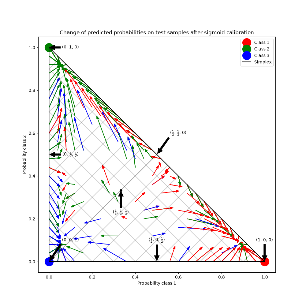Change of predicted probabilities on test samples after sigmoid calibration

In the figure above, each vertex of the simplex represents a perfectly predicted class (e.g., 1, 0, 0). The mid point inside the simplex represents predicting the three classes with equal probability (i.e., 1/3, 1/3, 1/3). Each arrow starts at the uncalibrated probabilities and end with the arrow head at the calibrated probability. The color of the arrow represents the true class of that test sample.

The uncalibrated classifier is overly confident in its predictions and incurs a large log loss. The calibrated classifier incurs a lower log loss due to two factors. First, notice in the figure above that the arrows generally point away from the edges of the simplex, where the probability of one class is 0. Second, a large proportion of the arrows point towards the true class, e.g., green arrows (samples where the true class is ‘green’) generally point towards the green vertex. This results in fewer over-confident, 0 predicted probabilities and at the same time an increase in the predicted probabilities of the correct class. Thus, the calibrated classifier produces more accurate predicted probabilities that incur a lower log loss

We can show this objectively by comparing the log loss of the uncalibrated and calibrated classifiers on the predictions of the 1000 test samples. Note that an alternative would have been to increase the number of base estimators (trees) of the RandomForestClassifier which would have resulted in a similar decrease in log loss.

from sklearn.metrics import log_loss

loss = log_loss(y_test, clf_probs)
cal_loss = log_loss(y_test, cal_clf_probs)

print("Log-loss of:")
print(f" - uncalibrated classifier: {loss:.3f}")
print(f" - calibrated classifier: {cal_loss:.3f}")

Log-loss of:
 - uncalibrated classifier: 1.327
 - calibrated classifier: 0.549

We can also assess calibration with the Brier score for probabilistics predictions (lower is better, possible range is [0, 2]):

from sklearn.metrics import brier_score_loss

loss = brier_score_loss(y_test, clf_probs)
cal_loss = brier_score_loss(y_test, cal_clf_probs)

print("Brier score of")
print(f" - uncalibrated classifier: {loss:.3f}")
print(f" - calibrated classifier: {cal_loss:.3f}")

Brier score of
 - uncalibrated classifier: 0.308
 - calibrated classifier: 0.310

According to the Brier score, the calibrated classifier is not better than the original model.

Finally we generate a grid of possible uncalibrated probabilities over the 2-simplex, compute the corresponding calibrated probabilities and plot arrows for each. The arrows are colored according the highest uncalibrated probability. This illustrates the learned calibration map:

plt.figure(figsize=(10, 10))
# Generate grid of probability values
p1d = np.linspace(0, 1, 20)
p0, p1 = np.meshgrid(p1d, p1d)
p2 = 1 - p0 - p1
p = np.c_[p0.ravel(), p1.ravel(), p2.ravel()]
p = p[p[:, 2] >= 0]

# Use the three class-wise calibrators to compute calibrated probabilities
calibrated_classifier = cal_clf.calibrated_classifiers_[0]
prediction = np.vstack(
    [
        calibrator.predict(this_p)
        for calibrator, this_p in zip(calibrated_classifier.calibrators, p.T)
    ]
).T

# Re-normalize the calibrated predictions to make sure they stay inside the
# simplex. This same renormalization step is performed internally by the
# predict method of CalibratedClassifierCV on multiclass problems.
prediction /= prediction.sum(axis=1)[:, None]

# Plot changes in predicted probabilities induced by the calibrators
for i in range(prediction.shape[0]):
    plt.arrow(
        p[i, 0],
        p[i, 1],
        prediction[i, 0] - p[i, 0],
        prediction[i, 1] - p[i, 1],
        head_width=1e-2,
        color=colors[np.argmax(p[i])],
    )

# Plot the boundaries of the unit simplex
plt.plot([0.0, 1.0, 0.0, 0.0], [0.0, 0.0, 1.0, 0.0], "k", label="Simplex")

plt.grid(False)
for x in [0.0, 0.1, 0.2, 0.3, 0.4, 0.5, 0.6, 0.7, 0.8, 0.9, 1.0]:
    plt.plot([0, x], [x, 0], "k", alpha=0.2)
    plt.plot([0, 0 + (1 - x) / 2], [x, x + (1 - x) / 2], "k", alpha=0.2)
    plt.plot([x, x + (1 - x) / 2], [0, 0 + (1 - x) / 2], "k", alpha=0.2)

plt.title("Learned sigmoid calibration map")
plt.xlabel("Probability class 1")
plt.ylabel("Probability class 2")
plt.xlim(-0.05, 1.05)
plt.ylim(-0.05, 1.05)

plt.show()

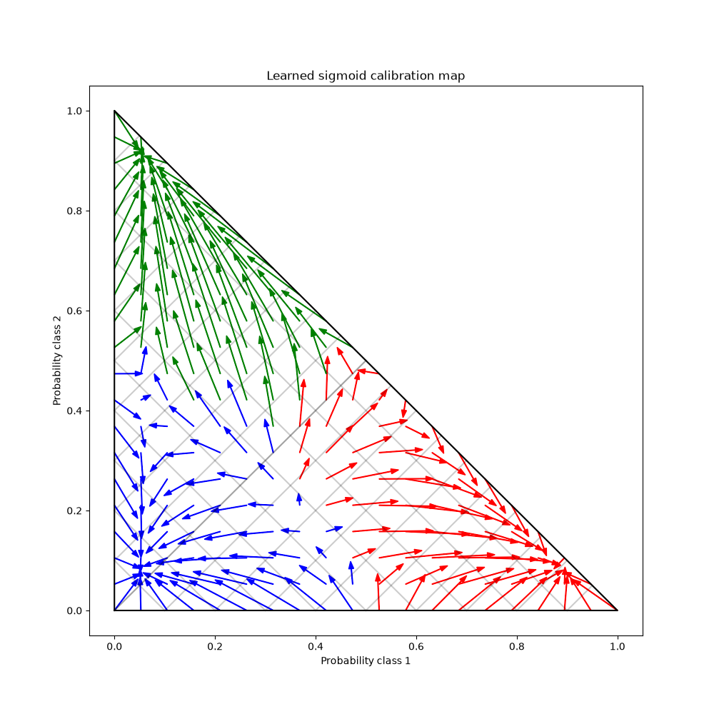One can observe that, on average, the calibrator is pushing highly confident predictions away from the boundaries of the simplex while simultaneously moving uncertain predictions towards one of three modes, one for each class. We can also observe that the mapping is not symmetric. Furthermore some arrows seem to cross class assignment boundaries which is not necessarily what one would expect from a calibration map as it means that some predicted classes will change after calibration.

All in all, the One-vs-Rest multiclass-calibration strategy implemented in CalibratedClassifierCV should not be trusted blindly.

Total running time of the script: (0 minutes 1.591 seconds)