GeezerVison is showing scikit-learn.org — Feature transformations with ensembles of trees
Note
Go to the end
to download the full example code or to run this example in your browser via JupyterLite or Binder.
Feature transformations with ensembles of trees#
Transform your features into a higher dimensional, sparse space. Then train a
linear model on these features.
First fit an ensemble of trees (totally random trees, a random forest, or
gradient boosted trees) on the training set. Then each leaf of each tree in the
ensemble is assigned a fixed arbitrary feature index in a new feature space.
These leaf indices are then encoded in a one-hot fashion.
Each sample goes through the decisions of each tree of the ensemble and ends up
in one leaf per tree. The sample is encoded by setting feature values for these
leaves to 1 and the other feature values to 0.
The resulting transformer has then learned a supervised, sparse,
high-dimensional categorical embedding of the data.
# Authors: The scikit-learn developers
# SPDX-License-Identifier: BSD-3-Clause
First, we will create a large dataset and split it into three sets:
a set to train the ensemble methods which are later used to as a feature
engineering transformer; a set to train the linear model; a set to test the linear model.
It is important to split the data in such way to avoid overfitting by leaking
data.
from sklearn.datasets import make_classification
from sklearn.model_selection import train_test_split

X, y = make_classification(n_samples=80_000, random_state=10)

X_full_train, X_test, y_full_train, y_test = train_test_split(
    X, y, test_size=0.5, random_state=10
)
X_train_ensemble, X_train_linear, y_train_ensemble, y_train_linear = train_test_split(
    X_full_train, y_full_train, test_size=0.5, random_state=10
)
For each of the ensemble methods, we will use 10 estimators and a maximum
depth of 3 levels.
n_estimators = 10
max_depth = 3
First, we will start by training the random forest and gradient boosting on
the separated training set
Notice that HistGradientBoostingClassifier is much
faster than GradientBoostingClassifier starting
with intermediate datasets (n_samples >= 10_000), which is not the case of
the present example.
The RandomTreesEmbedding is an unsupervised method
and thus does not required to be trained independently.
Now, we will create three pipelines that will use the above embedding as
a preprocessing stage.
The random trees embedding can be directly pipelined with the logistic
regression because it is a standard scikit-learn transformer.
Pipeline(steps=[('randomtreesembedding',
                 RandomTreesEmbedding(max_depth=3, n_estimators=10,
                                      random_state=0)),
                ('logisticregression', LogisticRegression(max_iter=1000))])
In a Jupyter environment, please rerun this cell to show the HTML representation or trust the notebook.
On GitHub, the HTML representation is unable to render, please try loading this page with nbviewer.org.
Parameters
|
steps
steps: list of tuples
List of (name of step, estimator) tuples that are to be chained in
sequential order. To be compatible with the scikit-learn API, all steps
must define `fit`. All non-last steps must also define `transform`. See
:ref:`Combining Estimators <combining_estimators>` for more details.
|
[('randomtreesembedding', ...), ('logisticregression', ...)] |
|
transform_input
transform_input: list of str, default=None
The names of the :term:`metadata` parameters that should be transformed by the
pipeline before passing it to the step consuming it.
This enables transforming some input arguments to ``fit`` (other than ``X``)
to be transformed by the steps of the pipeline up to the step which requires
them. Requirement is defined via :ref:`metadata routing <metadata_routing>`.
For instance, this can be used to pass a validation set through the pipeline.
You can only set this if metadata routing is enabled, which you
can enable using ``sklearn.set_config(enable_metadata_routing=True)``.
.. versionadded:: 1.6
|
None |
|
memory
memory: str or object with the joblib.Memory interface, default=None
Used to cache the fitted transformers of the pipeline. The last step
will never be cached, even if it is a transformer. By default, no
caching is performed. If a string is given, it is the path to the
caching directory. Enabling caching triggers a clone of the transformers
before fitting. Therefore, the transformer instance given to the
pipeline cannot be inspected directly. Use the attribute ``named_steps``
or ``steps`` to inspect estimators within the pipeline. Caching the
transformers is advantageous when fitting is time consuming. See
:ref:`sphx_glr_auto_examples_neighbors_plot_caching_nearest_neighbors.py`
for an example on how to enable caching.
|
None |
|
verbose
verbose: bool, default=False
If True, the time elapsed while fitting each step will be printed as it
is completed.
|
False |
Parameters
|
n_estimators
n_estimators: int, default=100
Number of trees in the forest.
.. versionchanged:: 0.22
The default value of ``n_estimators`` changed from 10 to 100
in 0.22.
|
10 |
|
max_depth
max_depth: int, default=5
The maximum depth of each tree. If None, then nodes are expanded until
all leaves are pure or until all leaves contain less than
min_samples_split samples.
|
3 |
|
random_state
random_state: int, RandomState instance or None, default=None
Controls the generation of the random `y` used to fit the trees
and the draw of the splits for each feature at the trees' nodes.
See :term:`Glossary <random_state>` for details.
|
0 |
|
min_samples_split
min_samples_split: int or float, default=2
The minimum number of samples required to split an internal node:
- If int, then consider `min_samples_split` as the minimum number.
- If float, then `min_samples_split` is a fraction and
`ceil(min_samples_split * n_samples)` is the minimum
number of samples for each split.
.. versionchanged:: 0.18
Added float values for fractions.
|
2 |
|
min_samples_leaf
min_samples_leaf: int or float, default=1
The minimum number of samples required to be at a leaf node.
A split point at any depth will only be considered if it leaves at
least ``min_samples_leaf`` training samples in each of the left and
right branches. This may have the effect of smoothing the model,
especially in regression.
- If int, then consider `min_samples_leaf` as the minimum number.
- If float, then `min_samples_leaf` is a fraction and
`ceil(min_samples_leaf * n_samples)` is the minimum
number of samples for each node.
.. versionchanged:: 0.18
Added float values for fractions.
|
1 |
|
min_weight_fraction_leaf
min_weight_fraction_leaf: float, default=0.0
The minimum weighted fraction of the sum total of weights (of all
the input samples) required to be at a leaf node. Samples have
equal weight when sample_weight is not provided.
|
0.0 |
|
max_leaf_nodes
max_leaf_nodes: int, default=None
Grow trees with ``max_leaf_nodes`` in best-first fashion.
Best nodes are defined as relative reduction in impurity.
If None then unlimited number of leaf nodes.
|
None |
|
min_impurity_decrease
min_impurity_decrease: float, default=0.0
A node will be split if this split induces a decrease of the impurity
greater than or equal to this value.
The weighted impurity decrease equation is the following::
N_t / N * (impurity - N_t_R / N_t * right_impurity
- N_t_L / N_t * left_impurity)
where ``N`` is the total number of samples, ``N_t`` is the number of
samples at the current node, ``N_t_L`` is the number of samples in the
left child, and ``N_t_R`` is the number of samples in the right child.
``N``, ``N_t``, ``N_t_R`` and ``N_t_L`` all refer to the weighted sum,
if ``sample_weight`` is passed.
.. versionadded:: 0.19
|
0.0 |
|
sparse_output
sparse_output: bool, default=True
Whether or not to return a sparse CSR matrix, as default behavior,
or to return a dense array compatible with dense pipeline operators.
|
True |
|
n_jobs
n_jobs: int, default=None
The number of jobs to run in parallel. :meth:`fit`, :meth:`transform`,
:meth:`decision_path` and :meth:`apply` are all parallelized over the
trees. ``None`` means 1 unless in a :obj:`joblib.parallel_backend`
context. ``-1`` means using all processors. See :term:`Glossary
<n_jobs>` for more details.
|
None |
|
verbose
verbose: int, default=0
Controls the verbosity when fitting and predicting.
|
0 |
|
warm_start
warm_start: bool, default=False
When set to ``True``, reuse the solution of the previous call to fit
and add more estimators to the ensemble, otherwise, just fit a whole
new forest. See :term:`Glossary <warm_start>` and
:ref:`tree_ensemble_warm_start` for details.
|
False |
Fitted attributes
| Name |
Type |
Value |
estimator_
estimator_: :class:`~sklearn.tree.ExtraTreeRegressor` instance
The child estimator template used to create the collection of fitted
sub-estimators.
.. versionadded:: 1.2
`base_estimator_` was renamed to `estimator_`.
|
ExtraTreeRegressor |
ExtraTreeRegressor() |
estimators_
estimators_: list of :class:`~sklearn.tree.ExtraTreeRegressor` instances
The collection of fitted sub-estimators.
|
list |
[ExtraTreeRegr...ate=209652396), ExtraTreeRegr...ate=398764591), ExtraTreeRegr...ate=924231285), ExtraTreeRegr...te=1478610112), ...] |
estimators_samples_
estimators_samples_: list of arrays
The subset of drawn samples (i.e., the in-bag samples) for each base
estimator. Each subset is defined by an array of the indices selected.
.. versionadded:: 1.4
|
list |
[array([ 0,..., dtype=int32), array([ 0,..., dtype=int32), array([ 0,..., dtype=int32), array([ 0,..., dtype=int32), ...] |
feature_importances_
feature_importances_: ndarray of shape (n_features,)
The feature importances (the higher, the more important the feature).
|
ndarray[float64](20,) |
[0.03,0.08,0. ,...,0.02,0.01,0.03] |
n_features_in_
n_features_in_: int
Number of features seen during :term:`fit`.
.. versionadded:: 0.24
|
int |
20 |
n_outputs_
n_outputs_: int
The number of outputs when ``fit`` is performed.
|
int |
1 |
one_hot_encoder_
one_hot_encoder_: OneHotEncoder instance
One-hot encoder used to create the sparse embedding.
|
OneHotEncoder |
OneHotEncoder() |
75 features
| randomtreesembedding_0_3 |
| randomtreesembedding_0_4 |
| randomtreesembedding_0_6 |
| randomtreesembedding_0_7 |
| randomtreesembedding_0_10 |
| randomtreesembedding_0_11 |
| randomtreesembedding_0_13 |
| randomtreesembedding_0_14 |
| randomtreesembedding_1_3 |
| randomtreesembedding_1_4 |
| randomtreesembedding_1_6 |
| randomtreesembedding_1_7 |
| randomtreesembedding_1_10 |
| randomtreesembedding_1_11 |
| randomtreesembedding_1_13 |
| randomtreesembedding_1_14 |
| randomtreesembedding_2_3 |
| randomtreesembedding_2_4 |
| randomtreesembedding_2_6 |
| randomtreesembedding_2_7 |
| randomtreesembedding_2_10 |
| randomtreesembedding_2_11 |
| randomtreesembedding_2_13 |
| randomtreesembedding_2_14 |
| randomtreesembedding_3_3 |
| randomtreesembedding_3_4 |
| randomtreesembedding_3_6 |
| randomtreesembedding_3_7 |
| randomtreesembedding_3_10 |
| randomtreesembedding_3_11 |
| randomtreesembedding_3_13 |
| randomtreesembedding_3_14 |
| randomtreesembedding_4_3 |
| randomtreesembedding_4_4 |
| randomtreesembedding_4_6 |
| randomtreesembedding_4_7 |
| randomtreesembedding_4_10 |
| randomtreesembedding_4_11 |
| randomtreesembedding_4_13 |
| randomtreesembedding_4_14 |
| randomtreesembedding_5_3 |
| randomtreesembedding_5_4 |
| randomtreesembedding_5_6 |
| randomtreesembedding_5_7 |
| randomtreesembedding_5_10 |
| randomtreesembedding_5_11 |
| randomtreesembedding_5_12 |
| randomtreesembedding_6_3 |
| randomtreesembedding_6_4 |
| randomtreesembedding_6_6 |
| randomtreesembedding_6_7 |
| randomtreesembedding_6_9 |
| randomtreesembedding_6_11 |
| randomtreesembedding_6_12 |
| randomtreesembedding_7_3 |
| randomtreesembedding_7_4 |
| randomtreesembedding_7_6 |
| randomtreesembedding_7_7 |
| randomtreesembedding_7_10 |
| randomtreesembedding_7_11 |
| randomtreesembedding_7_13 |
| randomtreesembedding_7_14 |
| randomtreesembedding_8_1 |
| randomtreesembedding_8_4 |
| randomtreesembedding_8_5 |
| randomtreesembedding_8_7 |
| randomtreesembedding_8_8 |
| randomtreesembedding_9_3 |
| randomtreesembedding_9_4 |
| randomtreesembedding_9_6 |
| randomtreesembedding_9_7 |
| randomtreesembedding_9_10 |
| randomtreesembedding_9_11 |
| randomtreesembedding_9_13 |
| randomtreesembedding_9_14 |
Parameters
|
max_iter
max_iter: int, default=100
Maximum number of iterations taken for the solvers to converge.
|
1000 |
|
penalty
penalty: {'l1', 'l2', 'elasticnet', None}, default='l2'
Specify the norm of the penalty:
- `None`: no penalty is added;
- `'l2'`: add an L2 penalty term and it is the default choice;
- `'l1'`: add an L1 penalty term;
- `'elasticnet'`: both L1 and L2 penalty terms are added.
.. warning::
Some penalties may not work with some solvers. See the parameter
`solver` below, to know the compatibility between the penalty and
solver.
.. versionadded:: 0.19
l1 penalty with SAGA solver (allowing 'multinomial' + L1)
.. deprecated:: 1.8
`penalty` was deprecated in version 1.8 and will be removed in 1.10.
Use `l1_ratio` and `C` instead. `l1_ratio=0` for `penalty='l2'`,
`l1_ratio=1` for `penalty='l1'`, `l1_ratio` set to any float between 0 and 1
for `penalty='elasticnet'`, and `C=np.inf` for `penalty=None`.
|
'deprecated' |
|
C
C: float, default=1.0
Inverse of regularization strength; must be a positive float.
Like in support vector machines, smaller values specify stronger
regularization. `C=np.inf` results in unpenalized logistic regression.
For a visual example on the effect of tuning the `C` parameter
with an L1 penalty, see:
:ref:`sphx_glr_auto_examples_linear_model_plot_logistic_path.py`.
|
1.0 |
|
l1_ratio
l1_ratio: float, default=0.0
The Elastic-Net mixing parameter, with `0 <= l1_ratio <= 1`. Setting
`l1_ratio=1` gives a pure L1-penalty, setting `l1_ratio=0` a pure L2-penalty.
Any value between 0 and 1 gives an Elastic-Net penalty of the form
`l1_ratio * L1 + (1 - l1_ratio) * L2`.
.. warning::
Certain values of `l1_ratio`, i.e. some penalties, may not work with some
solvers. See the parameter `solver` below, to know the compatibility between
the penalty and solver.
.. versionchanged:: 1.8
Default value changed from None to 0.0.
.. deprecated:: 1.8
`None` is deprecated and will be removed in version 1.10. Always use
`l1_ratio` to specify the penalty type.
|
0.0 |
|
dual
dual: bool, default=False
Dual (constrained) or primal (regularized, see also
:ref:`this equation <regularized-logistic-loss>`) formulation. Dual formulation
is only implemented for l2 penalty with liblinear solver. Prefer `dual=False`
when n_samples > n_features.
|
False |
|
tol
tol: float, default=1e-4
Tolerance for stopping criteria.
|
0.0001 |
|
fit_intercept
fit_intercept: bool, default=True
Specifies if a constant (a.k.a. bias or intercept) should be
added to the decision function.
|
True |
|
intercept_scaling
intercept_scaling: float, default=1
Useful only when the solver `liblinear` is used
and `self.fit_intercept` is set to `True`. In this case, `x` becomes
`[x, self.intercept_scaling]`,
i.e. a "synthetic" feature with constant value equal to
`intercept_scaling` is appended to the instance vector.
The intercept becomes
``intercept_scaling * synthetic_feature_weight``.
.. note::
The synthetic feature weight is subject to L1 or L2
regularization as all other features.
To lessen the effect of regularization on synthetic feature weight
(and therefore on the intercept) `intercept_scaling` has to be increased.
|
1 |
|
class_weight
class_weight: dict or 'balanced', default=None
Weights associated with classes in the form ``{class_label: weight}``.
If not given, all classes are supposed to have weight one.
The "balanced" mode uses the values of y to automatically adjust
weights inversely proportional to class frequencies in the input data
as ``n_samples / (n_classes * np.bincount(y))``.
Note that these weights will be multiplied with sample_weight (passed
through the fit method) if sample_weight is specified.
.. versionadded:: 0.17
*class_weight='balanced'*
|
None |
|
random_state
random_state: int, RandomState instance, default=None
Only used for `solver` == 'sag', 'saga' or 'liblinear' to shuffle the
data. It has no effect on the other solvers.
See :term:`Glossary <random_state>` for details.
|
None |
|
solver
solver: {'lbfgs', 'liblinear', 'newton-cg', 'newton-cholesky', 'sag', 'saga'}, default='lbfgs'
Algorithm to use in the optimization problem. Default is 'lbfgs'.
To choose a solver, you might want to consider the following aspects:
- 'lbfgs' is a good default solver because it works reasonably well for a wide
class of problems.
- For :term:`multiclass` problems (`n_classes >= 3`), all solvers except
'liblinear' minimize the full multinomial loss, 'liblinear' will raise an
error.
- 'newton-cholesky' is a good choice for
`n_samples` >> `n_features * n_classes`, especially with one-hot encoded
categorical features with rare categories. Be aware that the memory usage
of this solver has a quadratic dependency on `n_features * n_classes`
because it explicitly computes the full Hessian matrix.
- For small datasets, 'liblinear' is a good choice, whereas 'sag'
and 'saga' are faster for large ones;
- 'liblinear' can only handle binary classification by default. To apply a
one-versus-rest scheme for the multiclass setting one can wrap it with the
:class:`~sklearn.multiclass.OneVsRestClassifier`.
.. warning::
The choice of the algorithm depends on the penalty chosen (`l1_ratio=0`
for L2-penalty, `l1_ratio=1` for L1-penalty and `0 < l1_ratio < 1` for
Elastic-Net) and on (multinomial) multiclass support:
================= ======================== ======================
solver l1_ratio multinomial multiclass
================= ======================== ======================
'lbfgs' l1_ratio=0 yes
'liblinear' l1_ratio=1 or l1_ratio=0 no
'newton-cg' l1_ratio=0 yes
'newton-cholesky' l1_ratio=0 yes
'sag' l1_ratio=0 yes
'saga' 0<=l1_ratio<=1 yes
================= ======================== ======================
.. note::
'sag' and 'saga' fast convergence is only guaranteed on features
with approximately the same scale. You can preprocess the data with
a scaler from :mod:`sklearn.preprocessing`.
.. seealso::
Refer to the :ref:`User Guide <Logistic_regression>` for more
information regarding :class:`LogisticRegression` and more specifically the
:ref:`Table <logistic_regression_solvers>`
summarizing solver/penalty supports.
.. versionadded:: 0.17
Stochastic Average Gradient (SAG) descent solver. Multinomial support in
version 0.18.
.. versionadded:: 0.19
SAGA solver.
.. versionchanged:: 0.22
The default solver changed from 'liblinear' to 'lbfgs' in 0.22.
.. versionadded:: 1.2
newton-cholesky solver. Multinomial support in version 1.6.
|
'lbfgs' |
|
verbose
verbose: int, default=0
For the liblinear and lbfgs solvers set verbose to any positive
number for verbosity.
|
0 |
|
warm_start
warm_start: bool, default=False
When set to True, reuse the solution of the previous call to fit as
initialization, otherwise, just erase the previous solution.
Useless for liblinear solver. See :term:`the Glossary <warm_start>`.
.. versionadded:: 0.17
*warm_start* to support *lbfgs*, *newton-cg*, *sag*, *saga* solvers.
|
False |
|
n_jobs
n_jobs: int, default=None
Does not have any effect.
.. deprecated:: 1.8
`n_jobs` is deprecated in version 1.8 and will be removed in 1.10.
|
None |
Fitted attributes
| Name |
Type |
Value |
classes_
classes_: ndarray of shape (n_classes, )
A list of class labels known to the classifier.
|
ndarray[int64](2,) |
[0,1] |
coef_
coef_: ndarray or CSR matrix of shape (1, n_features) or (n_classes, n_features)
Coefficients of the features in the decision function.
`coef_` is of shape (1, n_features) when the given problem is binary.
By default, it will be created as a dense array, but can be turned to
sparse (CSR format) through :meth:`sparsify` (which can be beneficial
under L1 regularization when many coefficients are zero), and back to
dense through :meth:`densify`.
|
ndarray[float64](1, 75) |
[[-1.15,-0.58,-0.9 ,..., 0.32, 0.11, 0.24]] |
intercept_
intercept_: ndarray of shape (1,) or (n_classes,)
Intercept (a.k.a. bias) added to the decision function.
If `fit_intercept` is set to False, the intercept is set to zero.
`intercept_` is of shape (1,) when the given problem is binary.
|
ndarray[float64](1,) |
[0.35] |
n_features_in_
n_features_in_: int
Number of features seen during :term:`fit`.
.. versionadded:: 0.24
|
int |
75 |
n_iter_
n_iter_: ndarray of shape (1, )
Actual number of iterations for all classes.
.. versionchanged:: 0.20
In SciPy <= 1.0.0 the number of lbfgs iterations may exceed
``max_iter``. ``n_iter_`` will now report at most ``max_iter``.
|
ndarray[int32](1,) |
[36] |
Then, we can pipeline random forest or gradient boosting with a logistic
regression. However, the feature transformation will happen by calling the
method apply. The pipeline in scikit-learn expects a call to transform.
Therefore, we wrapped the call to apply within a FunctionTransformer.
Pipeline(steps=[('functiontransformer',
                 FunctionTransformer(func=<function rf_apply at 0x7e1dbc2a5170>,
                                     kw_args={'model': RandomForestClassifier(max_depth=3,
                                                                              n_estimators=10,
                                                                              random_state=10)})),
                ('onehotencoder', OneHotEncoder(handle_unknown='ignore')),
                ('logisticregression', LogisticRegression(max_iter=1000))])
In a Jupyter environment, please rerun this cell to show the HTML representation or trust the notebook.
On GitHub, the HTML representation is unable to render, please try loading this page with nbviewer.org.
Parameters
|
steps
steps: list of tuples
List of (name of step, estimator) tuples that are to be chained in
sequential order. To be compatible with the scikit-learn API, all steps
must define `fit`. All non-last steps must also define `transform`. See
:ref:`Combining Estimators <combining_estimators>` for more details.
|
[('functiontransformer', ...), ('onehotencoder', ...), ...] |
|
transform_input
transform_input: list of str, default=None
The names of the :term:`metadata` parameters that should be transformed by the
pipeline before passing it to the step consuming it.
This enables transforming some input arguments to ``fit`` (other than ``X``)
to be transformed by the steps of the pipeline up to the step which requires
them. Requirement is defined via :ref:`metadata routing <metadata_routing>`.
For instance, this can be used to pass a validation set through the pipeline.
You can only set this if metadata routing is enabled, which you
can enable using ``sklearn.set_config(enable_metadata_routing=True)``.
.. versionadded:: 1.6
|
None |
|
memory
memory: str or object with the joblib.Memory interface, default=None
Used to cache the fitted transformers of the pipeline. The last step
will never be cached, even if it is a transformer. By default, no
caching is performed. If a string is given, it is the path to the
caching directory. Enabling caching triggers a clone of the transformers
before fitting. Therefore, the transformer instance given to the
pipeline cannot be inspected directly. Use the attribute ``named_steps``
or ``steps`` to inspect estimators within the pipeline. Caching the
transformers is advantageous when fitting is time consuming. See
:ref:`sphx_glr_auto_examples_neighbors_plot_caching_nearest_neighbors.py`
for an example on how to enable caching.
|
None |
|
verbose
verbose: bool, default=False
If True, the time elapsed while fitting each step will be printed as it
is completed.
|
False |
rf_apply FunctionTransformer
Parameters
|
func
func: callable, default=None
The callable to use for the transformation. This will be passed
the same arguments as transform, with args and kwargs forwarded.
If func is None, then func will be the identity function.
|
<function rf_...x7e1dbc2a5170> |
|
kw_args
kw_args: dict, default=None
Dictionary of additional keyword arguments to pass to func.
.. versionadded:: 0.18
|
{'model': RandomForestC...ndom_state=10)} |
|
inverse_func
inverse_func: callable, default=None
The callable to use for the inverse transformation. This will be
passed the same arguments as inverse transform, with args and
kwargs forwarded. If inverse_func is None, then inverse_func
will be the identity function.
|
None |
|
validate
validate: bool, default=False
Indicate that the input X array should be checked before calling
``func``. The possibilities are:
- If False, there is no input validation.
- If True, then X will be converted to a 2-dimensional NumPy array or
sparse matrix. If the conversion is not possible an exception is
raised.
.. versionchanged:: 0.22
The default of ``validate`` changed from True to False.
|
False |
|
accept_sparse
accept_sparse: bool, default=False
Indicate that func accepts a sparse matrix as input. If validate is
False, this has no effect. Otherwise, if accept_sparse is false,
sparse matrix inputs will cause an exception to be raised.
|
False |
|
check_inverse
check_inverse: bool, default=True
Whether to check that or ``func`` followed by ``inverse_func`` leads to
the original inputs. It can be used for a sanity check, raising a
warning when the condition is not fulfilled.
.. versionadded:: 0.20
|
True |
|
feature_names_out
feature_names_out: callable, 'one-to-one' or None, default=None
Determines the list of feature names that will be returned by the
`get_feature_names_out` method. If it is 'one-to-one', then the output
feature names will be equal to the input feature names. If it is a
callable, then it must take two positional arguments: this
`FunctionTransformer` (`self`) and an array-like of input feature names
(`input_features`). It must return an array-like of output feature
names. The `get_feature_names_out` method is only defined if
`feature_names_out` is not None.
See ``get_feature_names_out`` for more details.
.. versionadded:: 1.1
|
None |
|
inv_kw_args
inv_kw_args: dict, default=None
Dictionary of additional keyword arguments to pass to inverse_func.
.. versionadded:: 0.18
|
None |
Parameters
|
handle_unknown
handle_unknown: {'error', 'ignore', 'infrequent_if_exist', 'warn'}, default='error'
Specifies the way unknown categories are handled during :meth:`transform`.
- 'error' : Raise an error if an unknown category is present during transform.
- 'ignore' : When an unknown category is encountered during
transform, the resulting one-hot encoded columns for this feature
will be all zeros. In the inverse transform, an unknown category
will be denoted as None.
- 'infrequent_if_exist' : When an unknown category is encountered
during transform, the resulting one-hot encoded columns for this
feature will map to the infrequent category if it exists. The
infrequent category will be mapped to the last position in the
encoding. During inverse transform, an unknown category will be
mapped to the category denoted `'infrequent'` if it exists. If the
`'infrequent'` category does not exist, then :meth:`transform` and
:meth:`inverse_transform` will handle an unknown category as with
`handle_unknown='ignore'`. Infrequent categories exist based on
`min_frequency` and `max_categories`. Read more in the
:ref:`User Guide <encoder_infrequent_categories>`.
- 'warn' : When an unknown category is encountered during transform
a warning is issued, and the encoding then proceeds as described for
`handle_unknown="infrequent_if_exist"`.
.. versionchanged:: 1.1
`'infrequent_if_exist'` was added to automatically handle unknown
categories and infrequent categories.
.. versionadded:: 1.6
The option `"warn"` was added in 1.6.
|
'ignore' |
|
categories
categories: 'auto' or a list of array-like, default='auto'
Categories (unique values) per feature:
- 'auto' : Determine categories automatically from the training data.
- list : ``categories[i]`` holds the categories expected in the ith
column. The passed categories should not mix strings and numeric
values within a single feature, and should be sorted in case of
numeric values.
The used categories can be found in the ``categories_`` attribute.
.. versionadded:: 0.20
|
'auto' |
|
drop
drop: {'first', 'if_binary'} or an array-like of shape (n_features,), default=None
Specifies a methodology to use to drop one of the categories per
feature. This is useful in situations where perfectly collinear
features cause problems, such as when feeding the resulting data
into an unregularized linear regression model.
However, dropping one category breaks the symmetry of the original
representation and can therefore induce a bias in downstream models,
for instance for penalized linear classification or regression models.
- None : retain all features (the default).
- 'first' : drop the first category in each feature. If only one
category is present, the feature will be dropped entirely.
- 'if_binary' : drop the first category in each feature with two
categories. Features with 1 or more than 2 categories are
left intact.
- array : ``drop[i]`` is the category in feature ``X[:, i]`` that
should be dropped.
When `max_categories` or `min_frequency` is configured to group
infrequent categories, the dropping behavior is handled after the
grouping.
.. versionadded:: 0.21
The parameter `drop` was added in 0.21.
.. versionchanged:: 0.23
The option `drop='if_binary'` was added in 0.23.
.. versionchanged:: 1.1
Support for dropping infrequent categories.
|
None |
|
sparse_output
sparse_output: bool, default=True
When ``True``, it returns a SciPy sparse matrix/array
in "Compressed Sparse Row" (CSR) format.
.. versionadded:: 1.2
`sparse` was renamed to `sparse_output`
|
True |
|
dtype
dtype: number type, default=np.float64
Desired dtype of output.
|
<class 'numpy.float64'> |
|
min_frequency
min_frequency: int or float, default=None
Specifies the minimum frequency below which a category will be
considered infrequent.
- If `int`, categories with a smaller cardinality will be considered
infrequent.
- If `float`, categories with a smaller cardinality than
`min_frequency * n_samples` will be considered infrequent.
.. versionadded:: 1.1
Read more in the :ref:`User Guide <encoder_infrequent_categories>`.
|
None |
|
max_categories
max_categories: int, default=None
Specifies an upper limit to the number of output features for each input
feature when considering infrequent categories. If there are infrequent
categories, `max_categories` includes the category representing the
infrequent categories along with the frequent categories. If `None`,
there is no limit to the number of output features.
.. versionadded:: 1.1
Read more in the :ref:`User Guide <encoder_infrequent_categories>`.
|
None |
|
feature_name_combiner
feature_name_combiner: "concat" or callable, default="concat"
Callable with signature `def callable(input_feature, category)` that returns a
string. This is used to create feature names to be returned by
:meth:`get_feature_names_out`.
`"concat"` concatenates encoded feature name and category with
`feature + "_" + str(category)`.E.g. feature X with values 1, 6, 7 create
feature names `X_1, X_6, X_7`.
.. versionadded:: 1.3
|
'concat' |
Fitted attributes
| Name |
Type |
Value |
categories_
categories_: list of arrays
The categories of each feature determined during fitting
(in order of the features in X and corresponding with the output
of ``transform``). This includes the category specified in ``drop``
(if any).
|
list |
[array([ 3, 4..., 11, 13, 14]), array([ 3, 4..., 11, 13, 14]), array([ 3, 4..., 11, 13, 14]), array([ 3, 4..., 11, 13, 14]), ...] |
drop_idx_
drop_idx_: array of shape (n_features,)
- ``drop_idx_[i]`` is the index in ``categories_[i]`` of the category
to be dropped for each feature.
- ``drop_idx_[i] = None`` if no category is to be dropped from the
feature with index ``i``, e.g. when `drop='if_binary'` and the
feature isn't binary.
- ``drop_idx_ = None`` if all the transformed features will be
retained.
If infrequent categories are enabled by setting `min_frequency` or
`max_categories` to a non-default value and `drop_idx[i]` corresponds
to an infrequent category, then the entire infrequent category is
dropped.
.. versionchanged:: 0.23
Added the possibility to contain `None` values.
|
NoneType |
None |
n_features_in_
n_features_in_: int
Number of features seen during :term:`fit`.
.. versionadded:: 1.0
|
int |
10 |
79 features
| x0_3 |
| x0_4 |
| x0_6 |
| x0_7 |
| x0_10 |
| x0_11 |
| x0_13 |
| x0_14 |
| x1_3 |
| x1_4 |
| x1_6 |
| x1_7 |
| x1_10 |
| x1_11 |
| x1_13 |
| x1_14 |
| x2_3 |
| x2_4 |
| x2_6 |
| x2_7 |
| x2_10 |
| x2_11 |
| x2_13 |
| x2_14 |
| x3_3 |
| x3_4 |
| x3_6 |
| x3_7 |
| x3_10 |
| x3_11 |
| x3_13 |
| x3_14 |
| x4_3 |
| x4_4 |
| x4_6 |
| x4_7 |
| x4_10 |
| x4_11 |
| x4_13 |
| x4_14 |
| x5_3 |
| x5_4 |
| x5_6 |
| x5_7 |
| x5_10 |
| x5_11 |
| x5_13 |
| x5_14 |
| x6_3 |
| x6_4 |
| x6_6 |
| x6_7 |
| x6_10 |
| x6_11 |
| x6_13 |
| x6_14 |
| x7_3 |
| x7_4 |
| x7_6 |
| x7_7 |
| x7_10 |
| x7_11 |
| x7_13 |
| x7_14 |
| x8_3 |
| x8_4 |
| x8_6 |
| x8_7 |
| x8_10 |
| x8_11 |
| x8_13 |
| x8_14 |
| x9_3 |
| x9_4 |
| x9_7 |
| x9_10 |
| x9_11 |
| x9_13 |
| x9_14 |
Parameters
|
max_iter
max_iter: int, default=100
Maximum number of iterations taken for the solvers to converge.
|
1000 |
|
penalty
penalty: {'l1', 'l2', 'elasticnet', None}, default='l2'
Specify the norm of the penalty:
- `None`: no penalty is added;
- `'l2'`: add an L2 penalty term and it is the default choice;
- `'l1'`: add an L1 penalty term;
- `'elasticnet'`: both L1 and L2 penalty terms are added.
.. warning::
Some penalties may not work with some solvers. See the parameter
`solver` below, to know the compatibility between the penalty and
solver.
.. versionadded:: 0.19
l1 penalty with SAGA solver (allowing 'multinomial' + L1)
.. deprecated:: 1.8
`penalty` was deprecated in version 1.8 and will be removed in 1.10.
Use `l1_ratio` and `C` instead. `l1_ratio=0` for `penalty='l2'`,
`l1_ratio=1` for `penalty='l1'`, `l1_ratio` set to any float between 0 and 1
for `penalty='elasticnet'`, and `C=np.inf` for `penalty=None`.
|
'deprecated' |
|
C
C: float, default=1.0
Inverse of regularization strength; must be a positive float.
Like in support vector machines, smaller values specify stronger
regularization. `C=np.inf` results in unpenalized logistic regression.
For a visual example on the effect of tuning the `C` parameter
with an L1 penalty, see:
:ref:`sphx_glr_auto_examples_linear_model_plot_logistic_path.py`.
|
1.0 |
|
l1_ratio
l1_ratio: float, default=0.0
The Elastic-Net mixing parameter, with `0 <= l1_ratio <= 1`. Setting
`l1_ratio=1` gives a pure L1-penalty, setting `l1_ratio=0` a pure L2-penalty.
Any value between 0 and 1 gives an Elastic-Net penalty of the form
`l1_ratio * L1 + (1 - l1_ratio) * L2`.
.. warning::
Certain values of `l1_ratio`, i.e. some penalties, may not work with some
solvers. See the parameter `solver` below, to know the compatibility between
the penalty and solver.
.. versionchanged:: 1.8
Default value changed from None to 0.0.
.. deprecated:: 1.8
`None` is deprecated and will be removed in version 1.10. Always use
`l1_ratio` to specify the penalty type.
|
0.0 |
|
dual
dual: bool, default=False
Dual (constrained) or primal (regularized, see also
:ref:`this equation <regularized-logistic-loss>`) formulation. Dual formulation
is only implemented for l2 penalty with liblinear solver. Prefer `dual=False`
when n_samples > n_features.
|
False |
|
tol
tol: float, default=1e-4
Tolerance for stopping criteria.
|
0.0001 |
|
fit_intercept
fit_intercept: bool, default=True
Specifies if a constant (a.k.a. bias or intercept) should be
added to the decision function.
|
True |
|
intercept_scaling
intercept_scaling: float, default=1
Useful only when the solver `liblinear` is used
and `self.fit_intercept` is set to `True`. In this case, `x` becomes
`[x, self.intercept_scaling]`,
i.e. a "synthetic" feature with constant value equal to
`intercept_scaling` is appended to the instance vector.
The intercept becomes
``intercept_scaling * synthetic_feature_weight``.
.. note::
The synthetic feature weight is subject to L1 or L2
regularization as all other features.
To lessen the effect of regularization on synthetic feature weight
(and therefore on the intercept) `intercept_scaling` has to be increased.
|
1 |
|
class_weight
class_weight: dict or 'balanced', default=None
Weights associated with classes in the form ``{class_label: weight}``.
If not given, all classes are supposed to have weight one.
The "balanced" mode uses the values of y to automatically adjust
weights inversely proportional to class frequencies in the input data
as ``n_samples / (n_classes * np.bincount(y))``.
Note that these weights will be multiplied with sample_weight (passed
through the fit method) if sample_weight is specified.
.. versionadded:: 0.17
*class_weight='balanced'*
|
None |
|
random_state
random_state: int, RandomState instance, default=None
Only used for `solver` == 'sag', 'saga' or 'liblinear' to shuffle the
data. It has no effect on the other solvers.
See :term:`Glossary <random_state>` for details.
|
None |
|
solver
solver: {'lbfgs', 'liblinear', 'newton-cg', 'newton-cholesky', 'sag', 'saga'}, default='lbfgs'
Algorithm to use in the optimization problem. Default is 'lbfgs'.
To choose a solver, you might want to consider the following aspects:
- 'lbfgs' is a good default solver because it works reasonably well for a wide
class of problems.
- For :term:`multiclass` problems (`n_classes >= 3`), all solvers except
'liblinear' minimize the full multinomial loss, 'liblinear' will raise an
error.
- 'newton-cholesky' is a good choice for
`n_samples` >> `n_features * n_classes`, especially with one-hot encoded
categorical features with rare categories. Be aware that the memory usage
of this solver has a quadratic dependency on `n_features * n_classes`
because it explicitly computes the full Hessian matrix.
- For small datasets, 'liblinear' is a good choice, whereas 'sag'
and 'saga' are faster for large ones;
- 'liblinear' can only handle binary classification by default. To apply a
one-versus-rest scheme for the multiclass setting one can wrap it with the
:class:`~sklearn.multiclass.OneVsRestClassifier`.
.. warning::
The choice of the algorithm depends on the penalty chosen (`l1_ratio=0`
for L2-penalty, `l1_ratio=1` for L1-penalty and `0 < l1_ratio < 1` for
Elastic-Net) and on (multinomial) multiclass support:
================= ======================== ======================
solver l1_ratio multinomial multiclass
================= ======================== ======================
'lbfgs' l1_ratio=0 yes
'liblinear' l1_ratio=1 or l1_ratio=0 no
'newton-cg' l1_ratio=0 yes
'newton-cholesky' l1_ratio=0 yes
'sag' l1_ratio=0 yes
'saga' 0<=l1_ratio<=1 yes
================= ======================== ======================
.. note::
'sag' and 'saga' fast convergence is only guaranteed on features
with approximately the same scale. You can preprocess the data with
a scaler from :mod:`sklearn.preprocessing`.
.. seealso::
Refer to the :ref:`User Guide <Logistic_regression>` for more
information regarding :class:`LogisticRegression` and more specifically the
:ref:`Table <logistic_regression_solvers>`
summarizing solver/penalty supports.
.. versionadded:: 0.17
Stochastic Average Gradient (SAG) descent solver. Multinomial support in
version 0.18.
.. versionadded:: 0.19
SAGA solver.
.. versionchanged:: 0.22
The default solver changed from 'liblinear' to 'lbfgs' in 0.22.
.. versionadded:: 1.2
newton-cholesky solver. Multinomial support in version 1.6.
|
'lbfgs' |
|
verbose
verbose: int, default=0
For the liblinear and lbfgs solvers set verbose to any positive
number for verbosity.
|
0 |
|
warm_start
warm_start: bool, default=False
When set to True, reuse the solution of the previous call to fit as
initialization, otherwise, just erase the previous solution.
Useless for liblinear solver. See :term:`the Glossary <warm_start>`.
.. versionadded:: 0.17
*warm_start* to support *lbfgs*, *newton-cg*, *sag*, *saga* solvers.
|
False |
|
n_jobs
n_jobs: int, default=None
Does not have any effect.
.. deprecated:: 1.8
`n_jobs` is deprecated in version 1.8 and will be removed in 1.10.
|
None |
Fitted attributes
| Name |
Type |
Value |
classes_
classes_: ndarray of shape (n_classes, )
A list of class labels known to the classifier.
|
ndarray[int64](2,) |
[0,1] |
coef_
coef_: ndarray or CSR matrix of shape (1, n_features) or (n_classes, n_features)
Coefficients of the features in the decision function.
`coef_` is of shape (1, n_features) when the given problem is binary.
By default, it will be created as a dense array, but can be turned to
sparse (CSR format) through :meth:`sparsify` (which can be beneficial
under L1 regularization when many coefficients are zero), and back to
dense through :meth:`densify`.
|
ndarray[float64](1, 79) |
[[ 0.15,-0.01, 0.59,...,-0.34, 0.7 ,-0.14]] |
intercept_
intercept_: ndarray of shape (1,) or (n_classes,)
Intercept (a.k.a. bias) added to the decision function.
If `fit_intercept` is set to False, the intercept is set to zero.
`intercept_` is of shape (1,) when the given problem is binary.
|
ndarray[float64](1,) |
[0.62] |
n_features_in_
n_features_in_: int
Number of features seen during :term:`fit`.
.. versionadded:: 0.24
|
int |
79 |
n_iter_
n_iter_: ndarray of shape (1, )
Actual number of iterations for all classes.
.. versionchanged:: 0.20
In SciPy <= 1.0.0 the number of lbfgs iterations may exceed
``max_iter``. ``n_iter_`` will now report at most ``max_iter``.
|
ndarray[int32](1,) |
[52] |
def gbdt_apply(X, model):
    return model.apply(X)[:, :, 0]


gbdt_leaves_yielder = FunctionTransformer(
    gbdt_apply, kw_args={"model": gradient_boosting}
)

gbdt_model = make_pipeline(
    gbdt_leaves_yielder,
    OneHotEncoder(handle_unknown="ignore"),
    LogisticRegression(max_iter=1000),
)
gbdt_model.fit(X_train_linear, y_train_linear)
Pipeline(steps=[('functiontransformer',
                 FunctionTransformer(func=<function gbdt_apply at 0x7e1dbc2a6ae0>,
                                     kw_args={'model': GradientBoostingClassifier(n_estimators=10,
                                                                                  random_state=10)})),
                ('onehotencoder', OneHotEncoder(handle_unknown='ignore')),
                ('logisticregression', LogisticRegression(max_iter=1000))])
In a Jupyter environment, please rerun this cell to show the HTML representation or trust the notebook.
On GitHub, the HTML representation is unable to render, please try loading this page with nbviewer.org.
Parameters
|
steps
steps: list of tuples
List of (name of step, estimator) tuples that are to be chained in
sequential order. To be compatible with the scikit-learn API, all steps
must define `fit`. All non-last steps must also define `transform`. See
:ref:`Combining Estimators <combining_estimators>` for more details.
|
[('functiontransformer', ...), ('onehotencoder', ...), ...] |
|
transform_input
transform_input: list of str, default=None
The names of the :term:`metadata` parameters that should be transformed by the
pipeline before passing it to the step consuming it.
This enables transforming some input arguments to ``fit`` (other than ``X``)
to be transformed by the steps of the pipeline up to the step which requires
them. Requirement is defined via :ref:`metadata routing <metadata_routing>`.
For instance, this can be used to pass a validation set through the pipeline.
You can only set this if metadata routing is enabled, which you
can enable using ``sklearn.set_config(enable_metadata_routing=True)``.
.. versionadded:: 1.6
|
None |
|
memory
memory: str or object with the joblib.Memory interface, default=None
Used to cache the fitted transformers of the pipeline. The last step
will never be cached, even if it is a transformer. By default, no
caching is performed. If a string is given, it is the path to the
caching directory. Enabling caching triggers a clone of the transformers
before fitting. Therefore, the transformer instance given to the
pipeline cannot be inspected directly. Use the attribute ``named_steps``
or ``steps`` to inspect estimators within the pipeline. Caching the
transformers is advantageous when fitting is time consuming. See
:ref:`sphx_glr_auto_examples_neighbors_plot_caching_nearest_neighbors.py`
for an example on how to enable caching.
|
None |
|
verbose
verbose: bool, default=False
If True, the time elapsed while fitting each step will be printed as it
is completed.
|
False |
gbdt_apply FunctionTransformer
Parameters
|
func
func: callable, default=None
The callable to use for the transformation. This will be passed
the same arguments as transform, with args and kwargs forwarded.
If func is None, then func will be the identity function.
|
<function gbd...x7e1dbc2a6ae0> |
|
kw_args
kw_args: dict, default=None
Dictionary of additional keyword arguments to pass to func.
.. versionadded:: 0.18
|
{'model': GradientBoost...ndom_state=10)} |
|
inverse_func
inverse_func: callable, default=None
The callable to use for the inverse transformation. This will be
passed the same arguments as inverse transform, with args and
kwargs forwarded. If inverse_func is None, then inverse_func
will be the identity function.
|
None |
|
validate
validate: bool, default=False
Indicate that the input X array should be checked before calling
``func``. The possibilities are:
- If False, there is no input validation.
- If True, then X will be converted to a 2-dimensional NumPy array or
sparse matrix. If the conversion is not possible an exception is
raised.
.. versionchanged:: 0.22
The default of ``validate`` changed from True to False.
|
False |
|
accept_sparse
accept_sparse: bool, default=False
Indicate that func accepts a sparse matrix as input. If validate is
False, this has no effect. Otherwise, if accept_sparse is false,
sparse matrix inputs will cause an exception to be raised.
|
False |
|
check_inverse
check_inverse: bool, default=True
Whether to check that or ``func`` followed by ``inverse_func`` leads to
the original inputs. It can be used for a sanity check, raising a
warning when the condition is not fulfilled.
.. versionadded:: 0.20
|
True |
|
feature_names_out
feature_names_out: callable, 'one-to-one' or None, default=None
Determines the list of feature names that will be returned by the
`get_feature_names_out` method. If it is 'one-to-one', then the output
feature names will be equal to the input feature names. If it is a
callable, then it must take two positional arguments: this
`FunctionTransformer` (`self`) and an array-like of input feature names
(`input_features`). It must return an array-like of output feature
names. The `get_feature_names_out` method is only defined if
`feature_names_out` is not None.
See ``get_feature_names_out`` for more details.
.. versionadded:: 1.1
|
None |
|
inv_kw_args
inv_kw_args: dict, default=None
Dictionary of additional keyword arguments to pass to inverse_func.
.. versionadded:: 0.18
|
None |
Parameters
|
handle_unknown
handle_unknown: {'error', 'ignore', 'infrequent_if_exist', 'warn'}, default='error'
Specifies the way unknown categories are handled during :meth:`transform`.
- 'error' : Raise an error if an unknown category is present during transform.
- 'ignore' : When an unknown category is encountered during
transform, the resulting one-hot encoded columns for this feature
will be all zeros. In the inverse transform, an unknown category
will be denoted as None.
- 'infrequent_if_exist' : When an unknown category is encountered
during transform, the resulting one-hot encoded columns for this
feature will map to the infrequent category if it exists. The
infrequent category will be mapped to the last position in the
encoding. During inverse transform, an unknown category will be
mapped to the category denoted `'infrequent'` if it exists. If the
`'infrequent'` category does not exist, then :meth:`transform` and
:meth:`inverse_transform` will handle an unknown category as with
`handle_unknown='ignore'`. Infrequent categories exist based on
`min_frequency` and `max_categories`. Read more in the
:ref:`User Guide <encoder_infrequent_categories>`.
- 'warn' : When an unknown category is encountered during transform
a warning is issued, and the encoding then proceeds as described for
`handle_unknown="infrequent_if_exist"`.
.. versionchanged:: 1.1
`'infrequent_if_exist'` was added to automatically handle unknown
categories and infrequent categories.
.. versionadded:: 1.6
The option `"warn"` was added in 1.6.
|
'ignore' |
|
categories
categories: 'auto' or a list of array-like, default='auto'
Categories (unique values) per feature:
- 'auto' : Determine categories automatically from the training data.
- list : ``categories[i]`` holds the categories expected in the ith
column. The passed categories should not mix strings and numeric
values within a single feature, and should be sorted in case of
numeric values.
The used categories can be found in the ``categories_`` attribute.
.. versionadded:: 0.20
|
'auto' |
|
drop
drop: {'first', 'if_binary'} or an array-like of shape (n_features,), default=None
Specifies a methodology to use to drop one of the categories per
feature. This is useful in situations where perfectly collinear
features cause problems, such as when feeding the resulting data
into an unregularized linear regression model.
However, dropping one category breaks the symmetry of the original
representation and can therefore induce a bias in downstream models,
for instance for penalized linear classification or regression models.
- None : retain all features (the default).
- 'first' : drop the first category in each feature. If only one
category is present, the feature will be dropped entirely.
- 'if_binary' : drop the first category in each feature with two
categories. Features with 1 or more than 2 categories are
left intact.
- array : ``drop[i]`` is the category in feature ``X[:, i]`` that
should be dropped.
When `max_categories` or `min_frequency` is configured to group
infrequent categories, the dropping behavior is handled after the
grouping.
.. versionadded:: 0.21
The parameter `drop` was added in 0.21.
.. versionchanged:: 0.23
The option `drop='if_binary'` was added in 0.23.
.. versionchanged:: 1.1
Support for dropping infrequent categories.
|
None |
|
sparse_output
sparse_output: bool, default=True
When ``True``, it returns a SciPy sparse matrix/array
in "Compressed Sparse Row" (CSR) format.
.. versionadded:: 1.2
`sparse` was renamed to `sparse_output`
|
True |
|
dtype
dtype: number type, default=np.float64
Desired dtype of output.
|
<class 'numpy.float64'> |
|
min_frequency
min_frequency: int or float, default=None
Specifies the minimum frequency below which a category will be
considered infrequent.
- If `int`, categories with a smaller cardinality will be considered
infrequent.
- If `float`, categories with a smaller cardinality than
`min_frequency * n_samples` will be considered infrequent.
.. versionadded:: 1.1
Read more in the :ref:`User Guide <encoder_infrequent_categories>`.
|
None |
|
max_categories
max_categories: int, default=None
Specifies an upper limit to the number of output features for each input
feature when considering infrequent categories. If there are infrequent
categories, `max_categories` includes the category representing the
infrequent categories along with the frequent categories. If `None`,
there is no limit to the number of output features.
.. versionadded:: 1.1
Read more in the :ref:`User Guide <encoder_infrequent_categories>`.
|
None |
|
feature_name_combiner
feature_name_combiner: "concat" or callable, default="concat"
Callable with signature `def callable(input_feature, category)` that returns a
string. This is used to create feature names to be returned by
:meth:`get_feature_names_out`.
`"concat"` concatenates encoded feature name and category with
`feature + "_" + str(category)`.E.g. feature X with values 1, 6, 7 create
feature names `X_1, X_6, X_7`.
.. versionadded:: 1.3
|
'concat' |
Fitted attributes
| Name |
Type |
Value |
categories_
categories_: list of arrays
The categories of each feature determined during fitting
(in order of the features in X and corresponding with the output
of ``transform``). This includes the category specified in ``drop``
(if any).
|
list |
[array([ 4., ...1., 13., 14.]), array([ 4., ...1., 13., 14.]), array([ 4., ...1., 13., 14.]), array([ 4., ...1., 13., 14.]), ...] |
drop_idx_
drop_idx_: array of shape (n_features,)
- ``drop_idx_[i]`` is the index in ``categories_[i]`` of the category
to be dropped for each feature.
- ``drop_idx_[i] = None`` if no category is to be dropped from the
feature with index ``i``, e.g. when `drop='if_binary'` and the
feature isn't binary.
- ``drop_idx_ = None`` if all the transformed features will be
retained.
If infrequent categories are enabled by setting `min_frequency` or
`max_categories` to a non-default value and `drop_idx[i]` corresponds
to an infrequent category, then the entire infrequent category is
dropped.
.. versionchanged:: 0.23
Added the possibility to contain `None` values.
|
NoneType |
None |
n_features_in_
n_features_in_: int
Number of features seen during :term:`fit`.
.. versionadded:: 1.0
|
int |
10 |
76 features
| x0_4.0 |
| x0_6.0 |
| x0_7.0 |
| x0_10.0 |
| x0_11.0 |
| x0_13.0 |
| x0_14.0 |
| x1_4.0 |
| x1_6.0 |
| x1_7.0 |
| x1_10.0 |
| x1_11.0 |
| x1_13.0 |
| x1_14.0 |
| x2_4.0 |
| x2_6.0 |
| x2_7.0 |
| x2_10.0 |
| x2_11.0 |
| x2_13.0 |
| x2_14.0 |
| x3_4.0 |
| x3_6.0 |
| x3_7.0 |
| x3_10.0 |
| x3_11.0 |
| x3_13.0 |
| x3_14.0 |
| x4_3.0 |
| x4_4.0 |
| x4_6.0 |
| x4_7.0 |
| x4_10.0 |
| x4_11.0 |
| x4_13.0 |
| x4_14.0 |
| x5_3.0 |
| x5_4.0 |
| x5_6.0 |
| x5_7.0 |
| x5_10.0 |
| x5_11.0 |
| x5_13.0 |
| x5_14.0 |
| x6_3.0 |
| x6_4.0 |
| x6_6.0 |
| x6_7.0 |
| x6_10.0 |
| x6_11.0 |
| x6_13.0 |
| x6_14.0 |
| x7_3.0 |
| x7_4.0 |
| x7_6.0 |
| x7_7.0 |
| x7_10.0 |
| x7_11.0 |
| x7_13.0 |
| x7_14.0 |
| x8_3.0 |
| x8_4.0 |
| x8_6.0 |
| x8_7.0 |
| x8_10.0 |
| x8_11.0 |
| x8_13.0 |
| x8_14.0 |
| x9_3.0 |
| x9_4.0 |
| x9_6.0 |
| x9_7.0 |
| x9_10.0 |
| x9_11.0 |
| x9_13.0 |
| x9_14.0 |
Parameters
|
max_iter
max_iter: int, default=100
Maximum number of iterations taken for the solvers to converge.
|
1000 |
|
penalty
penalty: {'l1', 'l2', 'elasticnet', None}, default='l2'
Specify the norm of the penalty:
- `None`: no penalty is added;
- `'l2'`: add an L2 penalty term and it is the default choice;
- `'l1'`: add an L1 penalty term;
- `'elasticnet'`: both L1 and L2 penalty terms are added.
.. warning::
Some penalties may not work with some solvers. See the parameter
`solver` below, to know the compatibility between the penalty and
solver.
.. versionadded:: 0.19
l1 penalty with SAGA solver (allowing 'multinomial' + L1)
.. deprecated:: 1.8
`penalty` was deprecated in version 1.8 and will be removed in 1.10.
Use `l1_ratio` and `C` instead. `l1_ratio=0` for `penalty='l2'`,
`l1_ratio=1` for `penalty='l1'`, `l1_ratio` set to any float between 0 and 1
for `penalty='elasticnet'`, and `C=np.inf` for `penalty=None`.
|
'deprecated' |
|
C
C: float, default=1.0
Inverse of regularization strength; must be a positive float.
Like in support vector machines, smaller values specify stronger
regularization. `C=np.inf` results in unpenalized logistic regression.
For a visual example on the effect of tuning the `C` parameter
with an L1 penalty, see:
:ref:`sphx_glr_auto_examples_linear_model_plot_logistic_path.py`.
|
1.0 |
|
l1_ratio
l1_ratio: float, default=0.0
The Elastic-Net mixing parameter, with `0 <= l1_ratio <= 1`. Setting
`l1_ratio=1` gives a pure L1-penalty, setting `l1_ratio=0` a pure L2-penalty.
Any value between 0 and 1 gives an Elastic-Net penalty of the form
`l1_ratio * L1 + (1 - l1_ratio) * L2`.
.. warning::
Certain values of `l1_ratio`, i.e. some penalties, may not work with some
solvers. See the parameter `solver` below, to know the compatibility between
the penalty and solver.
.. versionchanged:: 1.8
Default value changed from None to 0.0.
.. deprecated:: 1.8
`None` is deprecated and will be removed in version 1.10. Always use
`l1_ratio` to specify the penalty type.
|
0.0 |
|
dual
dual: bool, default=False
Dual (constrained) or primal (regularized, see also
:ref:`this equation <regularized-logistic-loss>`) formulation. Dual formulation
is only implemented for l2 penalty with liblinear solver. Prefer `dual=False`
when n_samples > n_features.
|
False |
|
tol
tol: float, default=1e-4
Tolerance for stopping criteria.
|
0.0001 |
|
fit_intercept
fit_intercept: bool, default=True
Specifies if a constant (a.k.a. bias or intercept) should be
added to the decision function.
|
True |
|
intercept_scaling
intercept_scaling: float, default=1
Useful only when the solver `liblinear` is used
and `self.fit_intercept` is set to `True`. In this case, `x` becomes
`[x, self.intercept_scaling]`,
i.e. a "synthetic" feature with constant value equal to
`intercept_scaling` is appended to the instance vector.
The intercept becomes
``intercept_scaling * synthetic_feature_weight``.
.. note::
The synthetic feature weight is subject to L1 or L2
regularization as all other features.
To lessen the effect of regularization on synthetic feature weight
(and therefore on the intercept) `intercept_scaling` has to be increased.
|
1 |
|
class_weight
class_weight: dict or 'balanced', default=None
Weights associated with classes in the form ``{class_label: weight}``.
If not given, all classes are supposed to have weight one.
The "balanced" mode uses the values of y to automatically adjust
weights inversely proportional to class frequencies in the input data
as ``n_samples / (n_classes * np.bincount(y))``.
Note that these weights will be multiplied with sample_weight (passed
through the fit method) if sample_weight is specified.
.. versionadded:: 0.17
*class_weight='balanced'*
|
None |
|
random_state
random_state: int, RandomState instance, default=None
Only used for `solver` == 'sag', 'saga' or 'liblinear' to shuffle the
data. It has no effect on the other solvers.
See :term:`Glossary <random_state>` for details.
|
None |
|
solver
solver: {'lbfgs', 'liblinear', 'newton-cg', 'newton-cholesky', 'sag', 'saga'}, default='lbfgs'
Algorithm to use in the optimization problem. Default is 'lbfgs'.
To choose a solver, you might want to consider the following aspects:
- 'lbfgs' is a good default solver because it works reasonably well for a wide
class of problems.
- For :term:`multiclass` problems (`n_classes >= 3`), all solvers except
'liblinear' minimize the full multinomial loss, 'liblinear' will raise an
error.
- 'newton-cholesky' is a good choice for
`n_samples` >> `n_features * n_classes`, especially with one-hot encoded
categorical features with rare categories. Be aware that the memory usage
of this solver has a quadratic dependency on `n_features * n_classes`
because it explicitly computes the full Hessian matrix.
- For small datasets, 'liblinear' is a good choice, whereas 'sag'
and 'saga' are faster for large ones;
- 'liblinear' can only handle binary classification by default. To apply a
one-versus-rest scheme for the multiclass setting one can wrap it with the
:class:`~sklearn.multiclass.OneVsRestClassifier`.
.. warning::
The choice of the algorithm depends on the penalty chosen (`l1_ratio=0`
for L2-penalty, `l1_ratio=1` for L1-penalty and `0 < l1_ratio < 1` for
Elastic-Net) and on (multinomial) multiclass support:
================= ======================== ======================
solver l1_ratio multinomial multiclass
================= ======================== ======================
'lbfgs' l1_ratio=0 yes
'liblinear' l1_ratio=1 or l1_ratio=0 no
'newton-cg' l1_ratio=0 yes
'newton-cholesky' l1_ratio=0 yes
'sag' l1_ratio=0 yes
'saga' 0<=l1_ratio<=1 yes
================= ======================== ======================
.. note::
'sag' and 'saga' fast convergence is only guaranteed on features
with approximately the same scale. You can preprocess the data with
a scaler from :mod:`sklearn.preprocessing`.
.. seealso::
Refer to the :ref:`User Guide <Logistic_regression>` for more
information regarding :class:`LogisticRegression` and more specifically the
:ref:`Table <logistic_regression_solvers>`
summarizing solver/penalty supports.
.. versionadded:: 0.17
Stochastic Average Gradient (SAG) descent solver. Multinomial support in
version 0.18.
.. versionadded:: 0.19
SAGA solver.
.. versionchanged:: 0.22
The default solver changed from 'liblinear' to 'lbfgs' in 0.22.
.. versionadded:: 1.2
newton-cholesky solver. Multinomial support in version 1.6.
|
'lbfgs' |
|
verbose
verbose: int, default=0
For the liblinear and lbfgs solvers set verbose to any positive
number for verbosity.
|
0 |
|
warm_start
warm_start: bool, default=False
When set to True, reuse the solution of the previous call to fit as
initialization, otherwise, just erase the previous solution.
Useless for liblinear solver. See :term:`the Glossary <warm_start>`.
.. versionadded:: 0.17
*warm_start* to support *lbfgs*, *newton-cg*, *sag*, *saga* solvers.
|
False |
|
n_jobs
n_jobs: int, default=None
Does not have any effect.
.. deprecated:: 1.8
`n_jobs` is deprecated in version 1.8 and will be removed in 1.10.
|
None |
Fitted attributes
| Name |
Type |
Value |
classes_
classes_: ndarray of shape (n_classes, )
A list of class labels known to the classifier.
|
ndarray[int64](2,) |
[0,1] |
coef_
coef_: ndarray or CSR matrix of shape (1, n_features) or (n_classes, n_features)
Coefficients of the features in the decision function.
`coef_` is of shape (1, n_features) when the given problem is binary.
By default, it will be created as a dense array, but can be turned to
sparse (CSR format) through :meth:`sparsify` (which can be beneficial
under L1 regularization when many coefficients are zero), and back to
dense through :meth:`densify`.
|
ndarray[float64](1, 76) |
[[-0.74, 0.11, 0.18,..., 0.55, 1.65,-3.16]] |
intercept_
intercept_: ndarray of shape (1,) or (n_classes,)
Intercept (a.k.a. bias) added to the decision function.
If `fit_intercept` is set to False, the intercept is set to zero.
`intercept_` is of shape (1,) when the given problem is binary.
|
ndarray[float64](1,) |
[-0.37] |
n_features_in_
n_features_in_: int
Number of features seen during :term:`fit`.
.. versionadded:: 0.24
|
int |
76 |
n_iter_
n_iter_: ndarray of shape (1, )
Actual number of iterations for all classes.
.. versionchanged:: 0.20
In SciPy <= 1.0.0 the number of lbfgs iterations may exceed
``max_iter``. ``n_iter_`` will now report at most ``max_iter``.
|
ndarray[int32](1,) |
[37] |
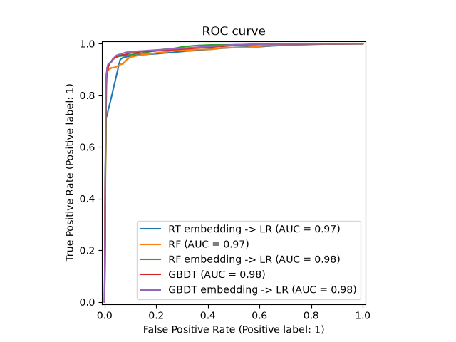
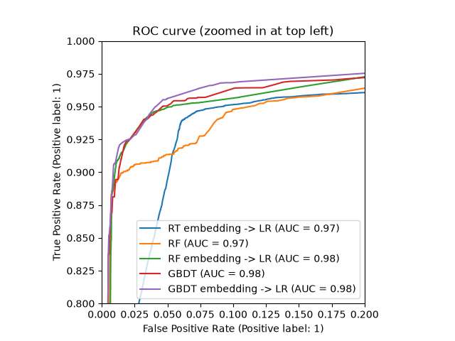
We can finally show the different ROC curves for all the models.
import matplotlib.pyplot as plt

from sklearn.metrics import RocCurveDisplay

_, ax = plt.subplots()

models = [
    ("RT embedding -> LR", rt_model),
    ("RF", random_forest),
    ("RF embedding -> LR", rf_model),
    ("GBDT", gradient_boosting),
    ("GBDT embedding -> LR", gbdt_model),
]

model_displays = {}
for name, pipeline in models:
    model_displays[name] = RocCurveDisplay.from_estimator(
        pipeline, X_test, y_test, ax=ax, name=name
    )
_ = ax.set_title("ROC curve")
 _, ax = plt.subplots()
for name, pipeline in models:
model_displays[name].plot(ax=ax)
ax.set_xlim(0, 0.2)
ax.set_ylim(0.8, 1)
_ = ax.set_title("ROC curve (zoomed in at top left)")
 Total running time of the script: (0 minutes 2.184 seconds)
Related examples
Gallery generated by Sphinx-Gallery
|