GeezerVison is showing scikit-learn.org — Decision Tree Regression
Note
Go to the end
to download the full example code or to run this example in your browser via JupyterLite or Binder.
Decision Tree Regression#
In this example, we demonstrate the effect of changing the maximum depth of a
decision tree on how it fits to the data. We perform this once on a 1D regression
task and once on a multi-output regression task.
# Authors: The scikit-learn developers
# SPDX-License-Identifier: BSD-3-Clause
Decision Tree on a 1D Regression Task#
Here we fit a tree on a 1D regression task.
The decision trees is
used to fit a sine curve with addition noisy observation. As a result, it
learns local linear regressions approximating the sine curve.
We can see that if the maximum depth of the tree (controlled by the
max_depth parameter) is set too high, the decision trees learn too fine
details of the training data and learn from the noise, i.e. they overfit.
Create a random 1D dataset#
Fit regression model#
Here we fit two models with different maximum depths
DecisionTreeRegressor(max_depth=5) In a Jupyter environment, please rerun this cell to show the HTML representation or trust the notebook.
On GitHub, the HTML representation is unable to render, please try loading this page with nbviewer.org.
Parameters
|
max_depth
max_depth: int, default=None
The maximum depth of the tree. If None, then nodes are expanded until
all leaves are pure or until all leaves contain less than
min_samples_split samples.
For an example of how ``max_depth`` influences the model, see
:ref:`sphx_glr_auto_examples_tree_plot_tree_regression.py`.
|
5 |
|
criterion
criterion: {"squared_error", "absolute_error", "poisson"}, default="squared_error"
The function to measure the quality of a split. Supported criteria
are "squared_error" for the mean squared error, which is equal to
variance reduction as feature selection criterion and minimizes the L2
loss using the mean of each terminal node, "absolute_error" for the mean
absolute error, which minimizes the L1 loss using the median of each terminal
node, and "poisson" which uses reduction in Poisson deviance to find splits,
also using the mean of each terminal node.
.. versionadded:: 0.18
Mean Absolute Error (MAE) criterion.
.. versionadded:: 0.24
Poisson deviance criterion.
.. versionchanged:: 1.9
Criterion `"friedman_mse"` was deprecated.
|
'squared_error' |
|
splitter
splitter: {"best", "random"}, default="best"
The strategy used to choose the split at each node. Supported
strategies are "best" to choose the best split and "random" to choose
the best random split among considered features for this split.
|
'best' |
|
min_samples_split
min_samples_split: int or float, default=2
The minimum number of samples required to split an internal node:
- If int, then consider `min_samples_split` as the minimum number.
- If float, then `min_samples_split` is a fraction and
`ceil(min_samples_split * n_samples)` are the minimum
number of samples for each split.
.. versionchanged:: 0.18
Added float values for fractions.
|
2 |
|
min_samples_leaf
min_samples_leaf: int or float, default=1
The minimum number of samples required to be at a leaf node.
A split point at any depth will only be considered if it leaves at
least ``min_samples_leaf`` training samples in each of the left and
right branches. This may have the effect of smoothing the model,
especially in regression.
- If int, then consider `min_samples_leaf` as the minimum number.
- If float, then `min_samples_leaf` is a fraction and
`ceil(min_samples_leaf * n_samples)` are the minimum
number of samples for each node.
.. versionchanged:: 0.18
Added float values for fractions.
|
1 |
|
min_weight_fraction_leaf
min_weight_fraction_leaf: float, default=0.0
The minimum weighted fraction of the sum total of weights (of all
the input samples) required to be at a leaf node. Samples have
equal weight when sample_weight is not provided.
|
0.0 |
|
max_features
max_features: int, float or {"sqrt", "log2"}, default=None
The number of features to consider when looking for the best split:
- If int, then consider `max_features` features at each split.
- If float, then `max_features` is a fraction and
`max(1, int(max_features * n_features_in_))` features are considered at each
split.
- If "sqrt", then `max_features=sqrt(n_features)`.
- If "log2", then `max_features=log2(n_features)`.
- If None, then `max_features=n_features`.
Note: splitting may inspect more than ``max_features`` features if
needed to find a valid split.
|
None |
|
random_state
random_state: int, RandomState instance or None, default=None
Controls the randomness of the estimator. The features are always
randomly permuted at each split, even if ``splitter`` is set to
``"best"``. When ``max_features < n_features``, the algorithm will
select ``max_features`` at random at each split before finding the best
split among them. But the best found split may vary across different
runs, even if ``max_features=n_features``. That is the case, if the
improvement of the criterion is identical for several splits and one
split has to be selected at random. To obtain a deterministic behaviour
during fitting, ``random_state`` has to be fixed to an integer.
See :term:`Glossary <random_state>` for details.
|
None |
|
max_leaf_nodes
max_leaf_nodes: int, default=None
Grow a tree with ``max_leaf_nodes`` in best-first fashion.
Best nodes are defined as relative reduction in impurity.
If None then unlimited number of leaf nodes.
|
None |
|
min_impurity_decrease
min_impurity_decrease: float, default=0.0
A node will be split if this split induces a decrease of the impurity
greater than or equal to this value.
The weighted impurity decrease equation is the following::
N_t / N * (impurity - N_t_R / N_t * right_impurity
- N_t_L / N_t * left_impurity)
where ``N`` is the total number of samples, ``N_t`` is the number of
samples at the current node, ``N_t_L`` is the number of samples in the
left child, and ``N_t_R`` is the number of samples in the right child.
``N``, ``N_t``, ``N_t_R`` and ``N_t_L`` all refer to the weighted sum,
if ``sample_weight`` is passed.
.. versionadded:: 0.19
|
0.0 |
|
ccp_alpha
ccp_alpha: non-negative float, default=0.0
Complexity parameter used for Minimal Cost-Complexity Pruning. The
subtree with the largest cost complexity that is smaller than
``ccp_alpha`` will be chosen. By default, no pruning is performed. See
:ref:`minimal_cost_complexity_pruning` for details. See
:ref:`sphx_glr_auto_examples_tree_plot_cost_complexity_pruning.py`
for an example of such pruning.
.. versionadded:: 0.22
|
0.0 |
|
monotonic_cst
monotonic_cst: array-like of int of shape (n_features), default=None
Indicates the monotonicity constraint to enforce on each feature.
- 1: monotonic increase
- 0: no constraint
- -1: monotonic decrease
If monotonic_cst is None, no constraints are applied.
Monotonicity constraints are not supported for:
- multioutput regressions (i.e. when `n_outputs_ > 1`).
Read more in the :ref:`User Guide <monotonic_cst_gbdt>`.
.. versionadded:: 1.4
|
None |
Predict#
Get predictions on the test set
X_test = np.arange(0.0, 5.0, 0.01)[:, np.newaxis]
y_1 = regr_1.predict(X_test)
y_2 = regr_2.predict(X_test)
Plot the results#
import matplotlib.pyplot as plt

plt.figure()
plt.scatter(X, y, s=20, edgecolor="black", c="darkorange", label="data")
plt.plot(X_test, y_1, color="cornflowerblue", label="max_depth=2", linewidth=2)
plt.plot(X_test, y_2, color="yellowgreen", label="max_depth=5", linewidth=2)
plt.xlabel("data")
plt.ylabel("target")
plt.title("Decision Tree Regression")
plt.legend()
plt.show()
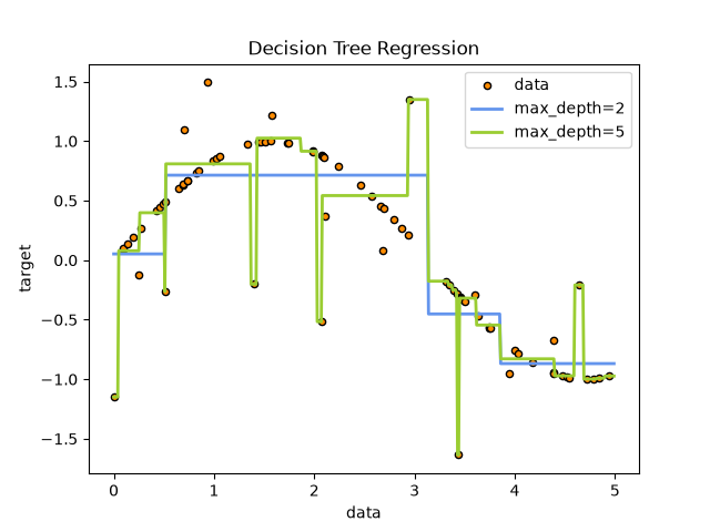 As you can see, the model with a depth of 5 (yellow) learns the details of the
training data to the point that it overfits to the noise. On the other hand,
the model with a depth of 2 (blue) learns the major tendencies in the data well
and does not overfit. In real use cases, you need to make sure that the tree
is not overfitting the training data, which can be done using cross-validation.
Decision Tree Regression with Multi-Output Targets#
Here the decision trees
is used to predict simultaneously the noisy x and y observations of a circle
given a single underlying feature. As a result, it learns local linear
regressions approximating the circle.
We can see that if the maximum depth of the tree (controlled by the
max_depth parameter) is set too high, the decision trees learn too fine
details of the training data and learn from the noise, i.e. they overfit.
Fit regression model#
DecisionTreeRegressor(max_depth=8) In a Jupyter environment, please rerun this cell to show the HTML representation or trust the notebook.
On GitHub, the HTML representation is unable to render, please try loading this page with nbviewer.org.
Parameters
|
max_depth
max_depth: int, default=None
The maximum depth of the tree. If None, then nodes are expanded until
all leaves are pure or until all leaves contain less than
min_samples_split samples.
For an example of how ``max_depth`` influences the model, see
:ref:`sphx_glr_auto_examples_tree_plot_tree_regression.py`.
|
8 |
|
criterion
criterion: {"squared_error", "absolute_error", "poisson"}, default="squared_error"
The function to measure the quality of a split. Supported criteria
are "squared_error" for the mean squared error, which is equal to
variance reduction as feature selection criterion and minimizes the L2
loss using the mean of each terminal node, "absolute_error" for the mean
absolute error, which minimizes the L1 loss using the median of each terminal
node, and "poisson" which uses reduction in Poisson deviance to find splits,
also using the mean of each terminal node.
.. versionadded:: 0.18
Mean Absolute Error (MAE) criterion.
.. versionadded:: 0.24
Poisson deviance criterion.
.. versionchanged:: 1.9
Criterion `"friedman_mse"` was deprecated.
|
'squared_error' |
|
splitter
splitter: {"best", "random"}, default="best"
The strategy used to choose the split at each node. Supported
strategies are "best" to choose the best split and "random" to choose
the best random split among considered features for this split.
|
'best' |
|
min_samples_split
min_samples_split: int or float, default=2
The minimum number of samples required to split an internal node:
- If int, then consider `min_samples_split` as the minimum number.
- If float, then `min_samples_split` is a fraction and
`ceil(min_samples_split * n_samples)` are the minimum
number of samples for each split.
.. versionchanged:: 0.18
Added float values for fractions.
|
2 |
|
min_samples_leaf
min_samples_leaf: int or float, default=1
The minimum number of samples required to be at a leaf node.
A split point at any depth will only be considered if it leaves at
least ``min_samples_leaf`` training samples in each of the left and
right branches. This may have the effect of smoothing the model,
especially in regression.
- If int, then consider `min_samples_leaf` as the minimum number.
- If float, then `min_samples_leaf` is a fraction and
`ceil(min_samples_leaf * n_samples)` are the minimum
number of samples for each node.
.. versionchanged:: 0.18
Added float values for fractions.
|
1 |
|
min_weight_fraction_leaf
min_weight_fraction_leaf: float, default=0.0
The minimum weighted fraction of the sum total of weights (of all
the input samples) required to be at a leaf node. Samples have
equal weight when sample_weight is not provided.
|
0.0 |
|
max_features
max_features: int, float or {"sqrt", "log2"}, default=None
The number of features to consider when looking for the best split:
- If int, then consider `max_features` features at each split.
- If float, then `max_features` is a fraction and
`max(1, int(max_features * n_features_in_))` features are considered at each
split.
- If "sqrt", then `max_features=sqrt(n_features)`.
- If "log2", then `max_features=log2(n_features)`.
- If None, then `max_features=n_features`.
Note: splitting may inspect more than ``max_features`` features if
needed to find a valid split.
|
None |
|
random_state
random_state: int, RandomState instance or None, default=None
Controls the randomness of the estimator. The features are always
randomly permuted at each split, even if ``splitter`` is set to
``"best"``. When ``max_features < n_features``, the algorithm will
select ``max_features`` at random at each split before finding the best
split among them. But the best found split may vary across different
runs, even if ``max_features=n_features``. That is the case, if the
improvement of the criterion is identical for several splits and one
split has to be selected at random. To obtain a deterministic behaviour
during fitting, ``random_state`` has to be fixed to an integer.
See :term:`Glossary <random_state>` for details.
|
None |
|
max_leaf_nodes
max_leaf_nodes: int, default=None
Grow a tree with ``max_leaf_nodes`` in best-first fashion.
Best nodes are defined as relative reduction in impurity.
If None then unlimited number of leaf nodes.
|
None |
|
min_impurity_decrease
min_impurity_decrease: float, default=0.0
A node will be split if this split induces a decrease of the impurity
greater than or equal to this value.
The weighted impurity decrease equation is the following::
N_t / N * (impurity - N_t_R / N_t * right_impurity
- N_t_L / N_t * left_impurity)
where ``N`` is the total number of samples, ``N_t`` is the number of
samples at the current node, ``N_t_L`` is the number of samples in the
left child, and ``N_t_R`` is the number of samples in the right child.
``N``, ``N_t``, ``N_t_R`` and ``N_t_L`` all refer to the weighted sum,
if ``sample_weight`` is passed.
.. versionadded:: 0.19
|
0.0 |
|
ccp_alpha
ccp_alpha: non-negative float, default=0.0
Complexity parameter used for Minimal Cost-Complexity Pruning. The
subtree with the largest cost complexity that is smaller than
``ccp_alpha`` will be chosen. By default, no pruning is performed. See
:ref:`minimal_cost_complexity_pruning` for details. See
:ref:`sphx_glr_auto_examples_tree_plot_cost_complexity_pruning.py`
for an example of such pruning.
.. versionadded:: 0.22
|
0.0 |
|
monotonic_cst
monotonic_cst: array-like of int of shape (n_features), default=None
Indicates the monotonicity constraint to enforce on each feature.
- 1: monotonic increase
- 0: no constraint
- -1: monotonic decrease
If monotonic_cst is None, no constraints are applied.
Monotonicity constraints are not supported for:
- multioutput regressions (i.e. when `n_outputs_ > 1`).
Read more in the :ref:`User Guide <monotonic_cst_gbdt>`.
.. versionadded:: 1.4
|
None |
Predict#
Get predictions on the test set
X_test = np.arange(-100.0, 100.0, 0.01)[:, np.newaxis]
y_1 = regr_1.predict(X_test)
y_2 = regr_2.predict(X_test)
y_3 = regr_3.predict(X_test)
Plot the results#
plt.figure()
s = 25
plt.scatter(y[:, 0], y[:, 1], c="yellow", s=s, edgecolor="black", label="data")
plt.scatter(
    y_1[:, 0],
    y_1[:, 1],
    c="cornflowerblue",
    s=s,
    edgecolor="black",
    label="max_depth=2",
)
plt.scatter(y_2[:, 0], y_2[:, 1], c="red", s=s, edgecolor="black", label="max_depth=5")
plt.scatter(y_3[:, 0], y_3[:, 1], c="blue", s=s, edgecolor="black", label="max_depth=8")
plt.xlim([-6, 6])
plt.ylim([-6, 6])
plt.xlabel("target 1")
plt.ylabel("target 2")
plt.title("Multi-output Decision Tree Regression")
plt.legend(loc="best")
plt.show()
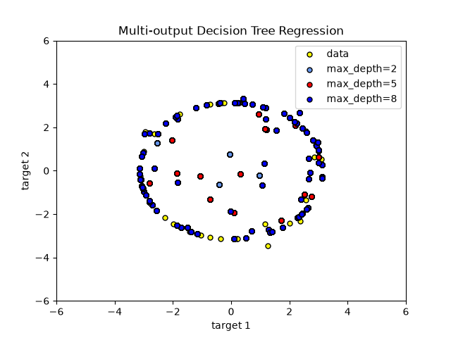 As you can see, the higher the value of max_depth, the more details of the data
are caught by the model. However, the model also overfits to the data and is
influenced by the noise.
Total running time of the script: (0 minutes 0.322 seconds)
Related examples
Gallery generated by Sphinx-Gallery
|