Note
Go to the end to download the full example code or to run this example in your browser via JupyterLite or Binder.
Plot multi-class SGD on the iris dataset#
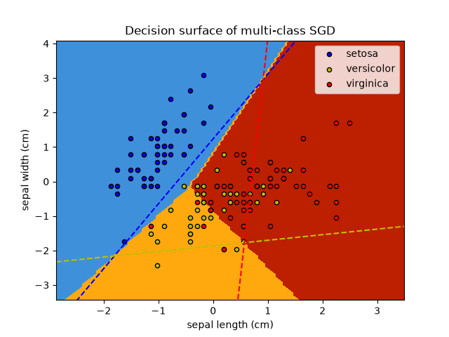
Plot decision surface of multi-class SGD on iris dataset. The hyperplanes corresponding to the three one-versus-all (OVA) classifiers are represented by the dashed lines.
# Authors: The scikit-learn developers
# SPDX-License-Identifier: BSD-3-Clause

import matplotlib.pyplot as plt
import numpy as np

from sklearn import datasets
from sklearn.inspection import DecisionBoundaryDisplay
from sklearn.linear_model import SGDClassifier

# import some data to play with
iris = datasets.load_iris()

# we only take the first two features. We could
# avoid this ugly slicing by using a two-dim dataset
X = iris.data[:, :2]
y = iris.target
colors = "byr"

# shuffle
idx = np.arange(X.shape[0])
np.random.seed(13)
np.random.shuffle(idx)
X = X[idx]
y = y[idx]

# standardize
mean = X.mean(axis=0)
std = X.std(axis=0)
X = (X - mean) / std

clf = SGDClassifier(alpha=0.001, max_iter=100).fit(X, y)
ax = plt.gca()
DecisionBoundaryDisplay.from_estimator(
    clf,
    X,
    ax=ax,
    response_method="predict",
    xlabel=iris.feature_names[0],
    ylabel=iris.feature_names[1],
)
plt.axis("tight")

# Plot also the training points
for i, color in zip(clf.classes_, colors):
    idx = (y == i).nonzero()
    plt.scatter(
        X[idx, 0],
        X[idx, 1],
        c=color,
        label=iris.target_names[i],
        edgecolor="black",
        s=20,
    )
plt.title("Decision surface of multi-class SGD")
plt.axis("tight")

# Plot the three one-against-all classifiers
xmin, xmax = plt.xlim()
ymin, ymax = plt.ylim()
coef = clf.coef_
intercept = clf.intercept_


def plot_hyperplane(c, color):
    def line(x0):
        return (-(x0 * coef[c, 0]) - intercept[c]) / coef[c, 1]

    plt.plot([xmin, xmax], [line(xmin), line(xmax)], ls="--", color=color)


for i, color in zip(clf.classes_, colors):
    plot_hyperplane(i, color)
plt.legend()
plt.show()
Total running time of the script: (0 minutes 0.117 seconds)


Related examples
Plot the decision surface of decision trees trained on the iris dataset
Plot the decision surface of decision trees trained on the iris dataset
Principal Component Analysis (PCA) on Iris Dataset
Principal Component Analysis (PCA) on Iris Dataset