Note

Go to the end to download the full example code or to run this example in your browser via JupyterLite or Binder.

Comparing Target Encoder with Other Encoders#

The TargetEncoder uses the value of the target to encode each categorical feature. In this example, we will compare three different approaches for handling categorical features: TargetEncoder, OrdinalEncoder, OneHotEncoder and dropping the category.

Note

fit(X, y).transform(X) does not equal fit_transform(X, y) because a cross fitting scheme is used in fit_transform for encoding. See the User Guide for details.

# Authors: The scikit-learn developers
# SPDX-License-Identifier: BSD-3-Clause

Loading Data from OpenML#

First, we load the wine reviews dataset, where the target is the points given be a reviewer:

from sklearn.datasets import fetch_openml

wine_reviews = fetch_openml(data_id=42074, as_frame=True)

df = wine_reviews.frame
df.head()

	country	description	designation	points	price	province	region_1	region_2	variety	winery
0	US	This tremendous 100% varietal wine hails from ...	Martha's Vineyard	96	235.0	California	Napa Valley	Napa	Cabernet Sauvignon	Heitz
1	Spain	Ripe aromas of fig, blackberry and cassis are ...	Carodorum Selección Especial Reserva	96	110.0	Northern Spain	Toro	NaN	Tinta de Toro	Bodega Carmen Rodríguez
2	US	Mac Watson honors the memory of a wine once ma...	Special Selected Late Harvest	96	90.0	California	Knights Valley	Sonoma	Sauvignon Blanc	Macauley
3	US	This spent 20 months in 30% new French oak, an...	Reserve	96	65.0	Oregon	Willamette Valley	Willamette Valley	Pinot Noir	Ponzi
4	France	This is the top wine from La Bégude, named aft...	La Brûlade	95	66.0	Provence	Bandol	NaN	Provence red blend	Domaine de la Bégude

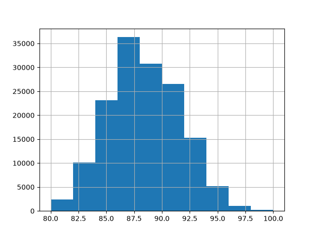
For this example, we use the following subset of numerical and categorical features in the data. The target are continuous values from 80 to 100:

numerical_features = ["price"]
categorical_features = [
    "country",
    "province",
    "region_1",
    "region_2",
    "variety",
    "winery",
]
target_name = "points"

X = df[numerical_features + categorical_features]
y = df[target_name]

_ = y.hist()

Training and Evaluating Pipelines with Different Encoders#

In this section, we will evaluate pipelines with HistGradientBoostingRegressor with different encoding strategies. First, we list out the encoders we will be using to preprocess the categorical features:

from sklearn.compose import ColumnTransformer
from sklearn.preprocessing import OneHotEncoder, OrdinalEncoder, TargetEncoder

categorical_preprocessors = [
    ("drop", "drop"),
    ("ordinal", OrdinalEncoder(handle_unknown="use_encoded_value", unknown_value=-1)),
    (
        "one_hot",
        OneHotEncoder(handle_unknown="ignore", max_categories=20, sparse_output=False),
    ),
    ("target", TargetEncoder(target_type="continuous")),
]

Next, we evaluate the models using cross validation and record the results:

from sklearn.ensemble import HistGradientBoostingRegressor
from sklearn.model_selection import cross_validate
from sklearn.pipeline import make_pipeline

n_cv_folds = 3
max_iter = 20
results = []


def evaluate_model_and_store(name, pipe):
    result = cross_validate(
        pipe,
        X,
        y,
        scoring="neg_root_mean_squared_error",
        cv=n_cv_folds,
        return_train_score=True,
    )
    rmse_test_score = -result["test_score"]
    rmse_train_score = -result["train_score"]
    results.append(
        {
            "preprocessor": name,
            "rmse_test_mean": rmse_test_score.mean(),
            "rmse_test_std": rmse_train_score.std(),
            "rmse_train_mean": rmse_train_score.mean(),
            "rmse_train_std": rmse_train_score.std(),
        }
    )


for name, categorical_preprocessor in categorical_preprocessors:
    preprocessor = ColumnTransformer(
        [
            ("numerical", "passthrough", numerical_features),
            ("categorical", categorical_preprocessor, categorical_features),
        ]
    )
    pipe = make_pipeline(
        preprocessor, HistGradientBoostingRegressor(random_state=0, max_iter=max_iter)
    )
    evaluate_model_and_store(name, pipe)

Native Categorical Feature Support#

In this section, we build and evaluate a pipeline that uses native categorical feature support in HistGradientBoostingRegressor, which only supports up to 255 unique categories. In our dataset, the most of the categorical features have more than 255 unique categories:

n_unique_categories = df[categorical_features].nunique().sort_values(ascending=False)
n_unique_categories

winery      14810
region_1     1236
variety       632
province      455
country        48
region_2       18
dtype: int64

To workaround the limitation above, we group the categorical features into low cardinality and high cardinality features. The high cardinality features will be target encoded and the low cardinality features will use the native categorical feature in gradient boosting.

high_cardinality_features = n_unique_categories[n_unique_categories > 255].index
low_cardinality_features = n_unique_categories[n_unique_categories <= 255].index
mixed_encoded_preprocessor = ColumnTransformer(
    [
        ("numerical", "passthrough", numerical_features),
        (
            "high_cardinality",
            TargetEncoder(target_type="continuous"),
            high_cardinality_features,
        ),
        (
            "low_cardinality",
            OrdinalEncoder(handle_unknown="use_encoded_value", unknown_value=-1),
            low_cardinality_features,
        ),
    ],
    verbose_feature_names_out=False,
)

# The output of the of the preprocessor must be set to pandas so the
# gradient boosting model can detect the low cardinality features.
mixed_encoded_preprocessor.set_output(transform="pandas")
mixed_pipe = make_pipeline(
    mixed_encoded_preprocessor,
    HistGradientBoostingRegressor(
        random_state=0, max_iter=max_iter, categorical_features=low_cardinality_features
    ),
)
mixed_pipe

Pipeline(steps=[('columntransformer',
                 ColumnTransformer(transformers=[('numerical', 'passthrough',
                                                  ['price']),
                                                 ('high_cardinality',
                                                  TargetEncoder(target_type='continuous'),
                                                  Index(['winery', 'region_1', 'variety', 'province'], dtype='str')),
                                                 ('low_cardinality',
                                                  OrdinalEncoder(handle_unknown='use_encoded_value',
                                                                 unknown_value=-1),
                                                  Index(['country', 'region_2'], dtype='str'))],
                                   verbose_feature_names_out=False)),
                ('histgradientboostingregressor',
                 HistGradientBoostingRegressor(categorical_features=Index(['country', 'region_2'], dtype='str'),
                                               max_iter=20, random_state=0))])

In a Jupyter environment, please rerun this cell to show the HTML representation or trust the notebook.
On GitHub, the HTML representation is unable to render, please try loading this page with nbviewer.org.

Pipeline

?Documentation for PipelineiNot fitted

Parameters

	steps steps: list of tuples List of (name of step, estimator) tuples that are to be chained in sequential order. To be compatible with the scikit-learn API, all steps must define `fit`. All non-last steps must also define `transform`. See :ref:`Combining Estimators <combining_estimators>` for more details.	[('columntransformer', ...), ('histgradientboostingregressor', ...)]
	transform_input transform_input: list of str, default=None The names of the :term:`metadata` parameters that should be transformed by the pipeline before passing it to the step consuming it. This enables transforming some input arguments to ``fit`` (other than ``X``) to be transformed by the steps of the pipeline up to the step which requires them. Requirement is defined via :ref:`metadata routing <metadata_routing>`. For instance, this can be used to pass a validation set through the pipeline. You can only set this if metadata routing is enabled, which you can enable using ``sklearn.set_config(enable_metadata_routing=True)``. .. versionadded:: 1.6	None
	memory memory: str or object with the joblib.Memory interface, default=None Used to cache the fitted transformers of the pipeline. The last step will never be cached, even if it is a transformer. By default, no caching is performed. If a string is given, it is the path to the caching directory. Enabling caching triggers a clone of the transformers before fitting. Therefore, the transformer instance given to the pipeline cannot be inspected directly. Use the attribute ``named_steps`` or ``steps`` to inspect estimators within the pipeline. Caching the transformers is advantageous when fitting is time consuming. See :ref:`sphx_glr_auto_examples_neighbors_plot_caching_nearest_neighbors.py` for an example on how to enable caching.	None
	verbose verbose: bool, default=False If True, the time elapsed while fitting each step will be printed as it is completed.	False

columntransformer: ColumnTransformer

?Documentation for columntransformer: ColumnTransformer

Parameters

	transformers transformers: list of tuples List of (name, transformer, columns) tuples specifying the transformer objects to be applied to subsets of the data. name : str Like in Pipeline and FeatureUnion, this allows the transformer and its parameters to be set using ``set_params`` and searched in grid search. transformer : {'drop', 'passthrough'} or estimator Estimator must support :term:`fit` and :term:`transform`. Special-cased strings 'drop' and 'passthrough' are accepted as well, to indicate to drop the columns or to pass them through untransformed, respectively. columns : str, array-like of str, int, array-like of int, array-like of bool, slice or callable Indexes the data on its second axis. Integers are interpreted as positional columns, while strings can reference DataFrame columns by name. A scalar string or int should be used where ``transformer`` expects X to be a 1d array-like (vector), otherwise a 2d array will be passed to the transformer. A callable is passed the input data `X` and can return any of the above. To select multiple columns by name or dtype, you can use :obj:`make_column_selector`.	[('numerical', ...), ('high_cardinality', ...), ...]
	verbose_feature_names_out verbose_feature_names_out: bool, str or Callable[[str, str], str], default=True - If True, :meth:`ColumnTransformer.get_feature_names_out` will prefix all feature names with the name of the transformer that generated that feature. It is equivalent to setting `verbose_feature_names_out="{transformer_name}__{feature_name}"`. - If False, :meth:`ColumnTransformer.get_feature_names_out` will not prefix any feature names and will error if feature names are not unique. - If ``Callable[[str, str], str]``, :meth:`ColumnTransformer.get_feature_names_out` will rename all the features using the name of the transformer. The first argument of the callable is the transformer name and the second argument is the feature name. The returned string will be the new feature name. - If ``str``, it must be a string ready for formatting. The given string will be formatted using two field names: ``transformer_name`` and ``feature_name``. e.g. ``"{feature_name}__{transformer_name}"``. See :meth:`str.format` method from the standard library for more info. .. versionadded:: 1.0 .. versionchanged:: 1.6 `verbose_feature_names_out` can be a callable or a string to be formatted.	False
	remainder remainder: {'drop', 'passthrough'} or estimator, default='drop' By default, only the specified columns in `transformers` are transformed and combined in the output, and the non-specified columns are dropped. (default of ``'drop'``). By specifying ``remainder='passthrough'``, all remaining columns that were not specified in `transformers`, but present in the data passed to `fit` will be automatically passed through. This subset of columns is concatenated with the output of the transformers. For dataframes, extra columns not seen during `fit` will be excluded from the output of `transform`. By setting ``remainder`` to be an estimator, the remaining non-specified columns will use the ``remainder`` estimator. The estimator must support :term:`fit` and :term:`transform`. Note that using this feature requires that the DataFrame columns input at :term:`fit` and :term:`transform` have identical order.	'drop'
	sparse_threshold sparse_threshold: float, default=0.3 If the output of the different transformers contains sparse matrices, these will be stacked as a sparse matrix if the overall density is lower than this value. Use ``sparse_threshold=0`` to always return dense. When the transformed output consists of all dense data, the stacked result will be dense, and this keyword will be ignored.	0.3
	n_jobs n_jobs: int, default=None Number of jobs to run in parallel. ``None`` means 1 unless in a :obj:`joblib.parallel_backend` context. ``-1`` means using all processors. See :term:`Glossary <n_jobs>` for more details.	None
	transformer_weights transformer_weights: dict, default=None Multiplicative weights for features per transformer. The output of the transformer is multiplied by these weights. Keys are transformer names, values the weights.	None
	verbose verbose: bool, default=False If True, the time elapsed while fitting each transformer will be printed as it is completed.	False

numerical

['price']

passthrough

high_cardinality

Index(['winery', 'region_1', 'variety', 'province'], dtype='str')

TargetEncoder

?Documentation for TargetEncoder

Parameters

	target_type target_type: {"auto", "continuous", "binary", "multiclass"}, default="auto" Type of target. - `"auto"` : Type of target is inferred with :func:`~sklearn.utils.multiclass.type_of_target`. - `"continuous"` : Continuous target - `"binary"` : Binary target - `"multiclass"` : Multiclass target .. note:: The type of target inferred with `"auto"` may not be the desired target type used for modeling. For example, if the target consisted of integers between 0 and 100, then :func:`~sklearn.utils.multiclass.type_of_target` will infer the target as `"multiclass"`. In this case, setting `target_type="continuous"` will specify the target as a regression problem. The `target_type_` attribute gives the target type used by the encoder. .. versionchanged:: 1.4 Added the option 'multiclass'.	'continuous'
	categories categories: "auto" or list of shape (n_features,) of array-like, default="auto" Categories (unique values) per feature: - `"auto"` : Determine categories automatically from the training data. - list : `categories[i]` holds the categories expected in the i-th column. The passed categories should not mix strings and numeric values within a single feature, and should be sorted in case of numeric values. The used categories are stored in the `categories_` fitted attribute.	'auto'
	smooth smooth: "auto" or float, default="auto" The amount of mixing of the target mean conditioned on the value of the category with the global target mean. A larger `smooth` value will put more weight on the global target mean. If `"auto"`, then `smooth` is set to an empirical Bayes estimate.	'auto'
	cv cv: int, cross-validation generator or an iterable, default=5 Determines the splitting strategy used in the internal :term:`cross fitting` during :meth:`fit_transform`. Splitters where each sample index doesn't appear in the validation fold exactly once, raise a `ValueError`. Possible inputs for cv are: - `None`, to use a 5-fold cross-validation chosen internally based on `target_type`, - integer, to specify the number of folds for the cross-validation chosen internally based on `target_type`, - :term:`CV splitter` that does not repeat samples across validation folds, - an iterable yielding (train, test) splits as arrays of indices. For integer/None inputs, if `target_type` is `"continuous"`, :class:`KFold` is used, otherwise :class:`StratifiedKFold` is used. Refer :ref:`User Guide <cross_validation>` for more information on cross-validation strategies. .. versionchanged:: 1.9 Cross-validation generators and iterables can also be passed as `cv`.	5
	shuffle shuffle: bool, default=True Whether to shuffle the data in :meth:`fit_transform` before splitting into folds. Note that the samples within each split will not be shuffled. Only applies if `cv` is an int or `None`. If `cv` is a cross-validation generator or an iterable, `shuffle` is ignored. .. deprecated:: 1.9 `shuffle` is deprecated and will be removed in 1.11. Pass a cross-validation generator as `cv` argument to specify the shuffling instead.	'deprecated'
	random_state random_state: int, RandomState instance or None, default=None When `shuffle` is True, `random_state` affects the ordering of the indices, which controls the randomness of each fold. Otherwise, this parameter has no effect. Pass an int for reproducible output across multiple function calls. See :term:`Glossary <random_state>`. .. deprecated:: 1.9 `random_state` is deprecated and will be removed in 1.11. Pass a cross-validation generator as `cv` argument to specify the random state of the shuffling instead.	'deprecated'

low_cardinality

Index(['country', 'region_2'], dtype='str')

OrdinalEncoder

?Documentation for OrdinalEncoder

Parameters

	handle_unknown handle_unknown: {'error', 'use_encoded_value'}, default='error' When set to 'error' an error will be raised in case an unknown categorical feature is present during transform. When set to 'use_encoded_value', the encoded value of unknown categories will be set to the value given for the parameter `unknown_value`. In :meth:`inverse_transform`, an unknown category will be denoted as None. .. versionadded:: 0.24	'use_encoded_value'
	unknown_value unknown_value: int or np.nan, default=None When the parameter handle_unknown is set to 'use_encoded_value', this parameter is required and will set the encoded value of unknown categories. It has to be distinct from the values used to encode any of the categories in `fit`. If set to np.nan, the `dtype` parameter must be a float dtype. .. versionadded:: 0.24	-1
	categories categories: 'auto' or a list of array-like, default='auto' Categories (unique values) per feature: - 'auto' : Determine categories automatically from the training data. - list : ``categories[i]`` holds the categories expected in the ith column. The passed categories should not mix strings and numeric values, and should be sorted in case of numeric values. The used categories can be found in the ``categories_`` attribute.	'auto'
	dtype dtype: number type, default=np.float64 Desired dtype of output.	<class 'numpy.float64'>
	encoded_missing_value encoded_missing_value: int or np.nan, default=np.nan Encoded value of missing categories. If set to `np.nan`, then the `dtype` parameter must be a float dtype. .. versionadded:: 1.1	nan
	min_frequency min_frequency: int or float, default=None Specifies the minimum frequency below which a category will be considered infrequent. - If `int`, categories with a smaller cardinality will be considered infrequent. - If `float`, categories with a smaller cardinality than `min_frequency * n_samples` will be considered infrequent. .. versionadded:: 1.3 Read more in the :ref:`User Guide <encoder_infrequent_categories>`.	None
	max_categories max_categories: int, default=None Specifies an upper limit to the number of output categories for each input feature when considering infrequent categories. If there are infrequent categories, `max_categories` includes the category representing the infrequent categories along with the frequent categories. If `None`, there is no limit to the number of output features. `max_categories` do not take into account missing or unknown categories. Setting `unknown_value` or `encoded_missing_value` to an integer will increase the number of unique integer codes by one each. This can result in up to `max_categories + 2` integer codes. .. versionadded:: 1.3 Read more in the :ref:`User Guide <encoder_infrequent_categories>`.	None

HistGradientBoostingRegressor

?Documentation for HistGradientBoostingRegressor

Parameters

	max_iter max_iter: int, default=100 The maximum number of iterations of the boosting process, i.e. the maximum number of trees.	20
	categorical_features categorical_features: array-like of {bool, int, str} of shape (n_features) or shape (n_categorical_features,), default='from_dtype' Indicates the categorical features. - None : no feature will be considered categorical. - boolean array-like : boolean mask indicating categorical features. - integer array-like : integer indices indicating categorical features. - str array-like: names of categorical features (assuming the training data has feature names). - `"from_dtype"`: dataframe columns with dtype "Categorical" and "Enum" are considered to be categorical features. The input must be a dataframe that is supported by narwhals (or supports it): :func:`narwhals.from_native` must work. This is the case, for instance, for pandas and polars DataFrames. For each categorical feature, there must be at most `max_bins` unique categories. Negative values for categorical features encoded as numeric dtypes are treated as missing values. All categorical values are converted to floating point numbers. This means that categorical values of 1.0 and 1 are treated as the same category. Read more in the :ref:`User Guide <categorical_support_gbdt>` and :ref:`sphx_glr_auto_examples_ensemble_plot_gradient_boosting_categorical.py`. .. versionadded:: 0.24 .. versionchanged:: 1.2 Added support for feature names. .. versionchanged:: 1.4 Added `"from_dtype"` option. .. versionchanged:: 1.6 The default value changed from `None` to `"from_dtype"`.	Index(['count..., dtype='str')
	random_state random_state: int, RandomState instance or None, default=None Pseudo-random number generator to control the subsampling in the binning process, and the train/validation data split if early stopping is enabled. Pass an int for reproducible output across multiple function calls. See :term:`Glossary <random_state>`.	0
	loss loss: {'squared_error', 'absolute_error', 'gamma', 'poisson', 'quantile'}, default='squared_error' The loss function to use in the boosting process. Note that the "squared error", "gamma" and "poisson" losses actually implement "half least squares loss", "half gamma deviance" and "half poisson deviance" to simplify the computation of the gradient. Furthermore, "gamma" and "poisson" losses internally use a log-link, "gamma" requires ``y > 0`` and "poisson" requires ``y >= 0``. "quantile" uses the pinball loss. .. versionchanged:: 0.23 Added option 'poisson'. .. versionchanged:: 1.1 Added option 'quantile'. .. versionchanged:: 1.3 Added option 'gamma'.	'squared_error'
	quantile quantile: float, default=None If loss is "quantile", this parameter specifies which quantile to be estimated and must be between 0 and 1.	None
	learning_rate learning_rate: float, default=0.1 The learning rate, also known as shrinkage. This is used as a multiplicative factor for the leaves values. Use ``1`` for no shrinkage.	0.1
	max_leaf_nodes max_leaf_nodes: int or None, default=31 The maximum number of leaves for each tree. Must be strictly greater than 1. If None, there is no maximum limit.	31
	max_depth max_depth: int or None, default=None The maximum depth of each tree. The depth of a tree is the number of edges to go from the root to the deepest leaf. Depth isn't constrained by default.	None
	min_samples_leaf min_samples_leaf: int, default=20 The minimum number of samples per leaf. For small datasets with less than a few hundred samples, it is recommended to lower this value since only very shallow trees would be built.	20
	l2_regularization l2_regularization: float, default=0 The L2 regularization parameter penalizing leaves with small hessians. Use ``0`` for no regularization (default).	0.0
	max_features max_features: float, default=1.0 Proportion of randomly chosen features in each and every node split. This is a form of regularization, smaller values make the trees weaker learners and might prevent overfitting. If interaction constraints from `interaction_cst` are present, only allowed features are taken into account for the subsampling. .. versionadded:: 1.4	1.0
	max_bins max_bins: int, default=255 The maximum number of bins to use for non-missing values. Before training, each feature of the input array `X` is binned into integer-valued bins, which allows for a much faster training stage. Features with a small number of unique values may use less than ``max_bins`` bins. In addition to the ``max_bins`` bins, one more bin is always reserved for missing values. Must be no larger than 255.	255
	monotonic_cst monotonic_cst: array-like of int of shape (n_features) or dict, default=None Monotonic constraint to enforce on each feature are specified using the following integer values: - 1: monotonic increase - 0: no constraint - -1: monotonic decrease If a dict with str keys, map feature to monotonic constraints by name. If an array, the features are mapped to constraints by position. See :ref:`monotonic_cst_features_names` for a usage example. Read more in the :ref:`User Guide <monotonic_cst_gbdt>`. .. versionadded:: 0.23 .. versionchanged:: 1.2 Accept dict of constraints with feature names as keys.	None
	interaction_cst interaction_cst: {"pairwise", "no_interactions"} or sequence of lists/tuples/sets of int, default=None Specify interaction constraints, the sets of features which can interact with each other in child node splits. Each item specifies the set of feature indices that are allowed to interact with each other. If there are more features than specified in these constraints, they are treated as if they were specified as an additional set. The strings "pairwise" and "no_interactions" are shorthands for allowing only pairwise or no interactions, respectively. For instance, with 5 features in total, `interaction_cst=[{0, 1}]` is equivalent to `interaction_cst=[{0, 1}, {2, 3, 4}]`, and specifies that each branch of a tree will either only split on features 0 and 1 or only split on features 2, 3 and 4. See :ref:`this example<ice-vs-pdp>` on how to use `interaction_cst`. .. versionadded:: 1.2	None
	warm_start warm_start: bool, default=False When set to ``True``, reuse the solution of the previous call to fit and add more estimators to the ensemble. For results to be valid, the estimator should be re-trained on the same data only. See :term:`the Glossary <warm_start>`.	False
	early_stopping early_stopping: 'auto' or bool, default='auto' If 'auto', early stopping is enabled if the sample size is larger than 10000 or if `X_val` and `y_val` are passed to `fit`. If True, early stopping is enabled, otherwise early stopping is disabled. .. versionadded:: 0.23	'auto'
	scoring scoring: str or callable or None, default='loss' Scoring method to use for early stopping. Only used if `early_stopping` is enabled. Options: - str: see :ref:`scoring_string_names` for options. - callable: a scorer callable object (e.g., function) with signature ``scorer(estimator, X, y)``. See :ref:`scoring_callable` for details. - `None`: the :ref:`coefficient of determination <r2_score>` (:math:`R^2`) is used. - 'loss': early stopping is checked w.r.t the loss value.	'loss'
	validation_fraction validation_fraction: int or float or None, default=0.1 Proportion (or absolute size) of training data to set aside as validation data for early stopping. If None, early stopping is done on the training data. The value is ignored if either early stopping is not performed, e.g. `early_stopping=False`, or if `X_val` and `y_val` are passed to fit.	0.1
	n_iter_no_change n_iter_no_change: int, default=10 Used to determine when to "early stop". The fitting process is stopped when none of the last ``n_iter_no_change`` scores are better than the ``n_iter_no_change - 1`` -th-to-last one, up to some tolerance. Only used if early stopping is performed.	10
	tol tol: float, default=1e-7 The absolute tolerance to use when comparing scores during early stopping. The higher the tolerance, the more likely we are to early stop: higher tolerance means that it will be harder for subsequent iterations to be considered an improvement upon the reference score.	1e-07
	verbose verbose: int, default=0 The verbosity level. If not zero, print some information about the fitting process. ``1`` prints only summary info, ``2`` prints info per iteration.	0

Finally, we evaluate the pipeline using cross validation and record the results:

evaluate_model_and_store("mixed_target", mixed_pipe)

Plotting the Results#

In this section, we display the results by plotting the test and train scores:

import matplotlib.pyplot as plt
import pandas as pd

results_df = (
    pd.DataFrame(results).set_index("preprocessor").sort_values("rmse_test_mean")
)

fig, (ax1, ax2) = plt.subplots(
    1, 2, figsize=(12, 8), sharey=True, constrained_layout=True
)
xticks = range(len(results_df))
name_to_color = dict(
    zip((r["preprocessor"] for r in results), ["C0", "C1", "C2", "C3", "C4"])
)

for subset, ax in zip(["test", "train"], [ax1, ax2]):
    mean, std = f"rmse_{subset}_mean", f"rmse_{subset}_std"
    data = results_df[[mean, std]].sort_values(mean)
    ax.bar(
        x=xticks,
        height=data[mean],
        yerr=data[std],
        width=0.9,
        color=[name_to_color[name] for name in data.index],
    )
    ax.set(
        title=f"RMSE ({subset.title()})",
        xlabel="Encoding Scheme",
        xticks=xticks,
        xticklabels=data.index,
    )

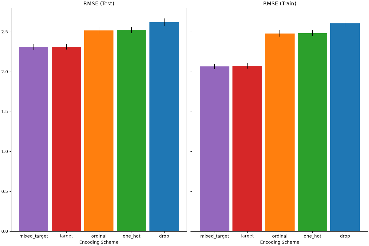When evaluating the predictive performance on the test set, dropping the categories perform the worst and the target encoders performs the best. This can be explained as follows:

Dropping the categorical features makes the pipeline less expressive and underfitting as a result;
Due to the high cardinality and to reduce the training time, the one-hot encoding scheme uses max_categories=20 which prevents the features from expanding too much, which can result in underfitting.
If we had not set max_categories=20, the one-hot encoding scheme would have likely made the pipeline overfitting as the number of features explodes with rare category occurrences that are correlated with the target by chance (on the training set only);
The ordinal encoding imposes an arbitrary order to the features which are then treated as numerical values by the HistGradientBoostingRegressor. Since this model groups numerical features in 256 bins per feature, many unrelated categories can be grouped together and as a result overall pipeline can underfit;
When using the target encoder, the same binning happens, but since the encoded values are statistically ordered by marginal association with the target variable, the binning use by the HistGradientBoostingRegressor makes sense and leads to good results: the combination of smoothed target encoding and binning works as a good regularizing strategy against overfitting while not limiting the expressiveness of the pipeline too much.