Part III Differentiating through programs

Chapter 7Finite differences

One of the simplest ways to numerically compute derivatives is to use finite differences, which approximate the infinitesimal definition of derivatives. Finite differences only require function evaluations, and can therefore work with blackbox functions: they ignore the compositional structure of functions. Without loss of generality, our exposition focuses on computing directional derivatives $\partial f (w) [v]$ ∂f(w)[v], for a function $f ⁣ : E \to F$ f:E→F, evaluated at $w \in E$ w∈E, in the direction $v \in E$ v∈E.

7.1 Forward differences

From Definition 2.4 and Definition 2.13, the directional derivative and more generally the JVP are defined as a limit, $\partial f (w) [v] ≔ \lim_{δ \to 0} \frac{f (w + δ v) - f (w)}{δ} .$ ∂f(w)[v]:=δ→0limδf(w+δv)−f(w). This suggests that we can approximate the directional derivative and the JVP using $\partial f (w) [v] \approx \frac{f (w + δ v) - f (w)}{δ},$ ∂f(w)[v]≈δf(w+δv)−f(w), for some $0 < δ ≪ 1$ 0<δ≪1. This formula is called a forward difference.

To measure the error incurred by this approximation, we use Landau’s $O$ O notation.

Remark 7.1 (Big $O$ O notation)

For two functions $g$ g and $f$ f, we write $g (δ) = O (f (δ)) as δ \to γ,$ g(δ)=O(f(δ)) as δ→γ, if the ratio $∣ g (δ) ∣ / ∣ f (δ) ∣$ ∣g(δ)∣/∣f(δ)∣ is bounded as $δ \to γ$ δ→γ. For example, we write $δ \cos (δ) = O (δ)$ δcos(δ)=O(δ) as $δ \to 0$ δ→0. In the following, unless otherwise specified, we compare limits as $δ \to 0$ δ→0. We observe that $g (δ) = O (δ^{k})$ g(δ)=O(δk) implies $g (δ) = o (δ^{k - 1})$ g(δ)=o(δk−1). However, Landau’s $O$ O notation provides finer practical interpretations than Landau’s $o$ o notation. For example, if $g (δ) = O (δ^{2})$ g(δ)=O(δ2), then we know its upper bound scales quadratically, meaning that reducing $δ$ δ by a factor of 2 reduces this bound by a factor of 4. Knowing only that $g (δ) = o (δ)$ g(δ)=o(δ) does not allow us to make such a concrete statement, because it merely dictates that $g (δ)$ g(δ) decays strictly faster than $δ$ δ, without providing a specific bounding rate or scaling factor for that decay. For numerical analysis, Landau’s $O$ O notation is therefore preferable.

From the Taylor expansion in Section 2.5.4, we indeed have $f (w + δ v) - f (w) = δ \partial f (w) [v] + \frac{δ^{2}}{2} \partial^{2} f (w) [v, v] + \frac{δ^{3}}{3!} \partial^{3} f (w) [v, v, v] + \dots$ f(w+δv)−f(w)=δ∂f(w)[v]+2δ2∂2f(w)[v,v]+3!δ3∂3f(w)[v,v,v]+… so that $\begin{matrix} \frac{f (w + δ v) - f (w)}{δ} & = \partial f (w) [v] + \frac{δ}{2} \partial^{2} f (w) [v, v] + \frac{δ^{2}}{3!} \partial^{3} f (w) [v, v, v] + \dots \\ = \partial f (w) [v] + O (δ) . \end{matrix}$ δf(w+δv)−f(w)=∂f(w)[v]+2δ∂2f(w)[v,v]+3!δ2∂3f(w)[v,v,v]+…=∂f(w)[v]+O(δ). The error incurred by choosing a finite rather than infinitesimal $δ$ δ in the forward difference formula is called the truncation error. The Taylor approximation above shows that this error is of the order of $O (δ)$ O(δ).

However, we cannot choose a too small value of $δ$ δ, because the evaluation of the function $f$ f on a computer rounds the value of $f$ f to machine precision. Mathematically, a scalar-valued function $f$ f evaluated on a computer becomes a function $\tilde{f}$ f~ such that $\tilde{f} (w) \approx [f (w) / ε] ε$ f~(w)≈[f(w)/ε]ε, where $[f (w) / ε]$ [f(w)/ε] denotes the closest integer of $f (w) / ε \in R$ f(w)/ε∈R and $ε$ ε is the machine precision, i.e., the smallest non-zero real number encoded by the machine. This means that the difference $f (w + δ v) - f (w)$ f(w+δv)−f(w) evaluated on a computer is prone to round-off error of the order of $O (ε)$ O(ε). We illustrate the trade-off between truncation and round-off errors in Fig. 7.1.

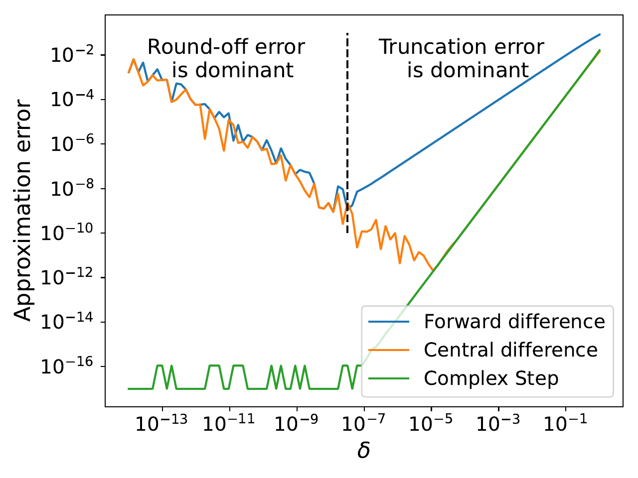
Figure 7.1: Numerical differentiation of $f (x) ≔ s o f t p l u s (x) = \log (1 + \exp (x))$ f(x):=softplus(x)=log(1+exp(x)), to approximate $f^{'} (x) = l o g i s t i c (x)$ f′(x)=logistic(x) at $x = 1$ x=1. The forward and central difference methods induce both truncation error (for large $δ$ δ) and round-off error (for small $δ$ δ). The complex step method enjoys smaller round-off error.

7.2 Backward differences

As an alternative, we can approximate the directional derivative and the JVP by $\partial f (w) [v] \approx \frac{f (w) - f (w - δ v)}{δ},$ ∂f(w)[v]≈δf(w)−f(w−δv), for some $0 < δ ≪ 1$ 0<δ≪1. This formula is called a backward difference. From the Taylor expansion in Section 2.5.4, we easily verify that $(f (w) - f (w - δ v)) / δ = \partial f (w) [v] + O (δ)$ (f(w)−f(w−δv))/δ=∂f(w)[v]+O(δ), so that the truncation error is the same as for the forward difference.

7.3 Central differences

Rather than using an asymmetric formula to approximate the derivative, as in forward and backward differences, we can use a symmetric formula $\partial f (w) [v] \approx \frac{f (w + δ v) - f (w - δ v)}{2 δ},$ ∂f(w)[v]≈2δf(w+δv)−f(w−δv), for some $0 < δ ≪ 1$ 0<δ≪1. This formula is called a central difference. From the Taylor expansion in Section 2.5.4, we have $\begin{matrix} f (w + δ v) - f (w - δ v) = & 2 δ \partial f (w) [v] + \frac{2 δ^{3}}{3!} \partial^{3} f (w) [v, v, v] \\ + \frac{2 δ^{5}}{5!} \partial^{5} f (w) [v, \dots, v] + \dots \end{matrix}$ f(w+δv)−f(w−δv)=2δ∂f(w)[v]+3!2δ3∂3f(w)[v,v,v]+5!2δ5∂5f(w)[v,…,v]+… so that $\begin{matrix} \frac{f (w + δ v) - f (w - δ v)}{2 δ} = & \partial f (w) [v] + \frac{δ^{2}}{3!} \partial^{3} f (w) [v, v, v] + \dots \\ = & \partial f (w) [v] + O (δ^{2}) . \end{matrix}$ 2δf(w+δv)−f(w−δv)==∂f(w)[v]+3!δ2∂3f(w)[v,v,v]+…∂f(w)[v]+O(δ2). We see that the terms corresponding to derivatives of even order canceled out, allowing the formula to achieve $O (δ^{2})$ O(δ2) truncation error. For any $δ < 1$ δ<1, the truncation error of the central difference is much smaller than the one of the forward or backward differences as confirmed empirically in Fig. 7.1.

7.4 Higher-accuracy finite differences

The truncation error can be further reduced by making use of additional function evaluations. One can generalize the forward difference scheme by a formula of the form $\partial f (w) [v] \approx \sum_{t = 0}^{p} \frac{a_{t}}{δ} f (w + t δ v)$ ∂f(w)[v]≈t=0∑pδatf(w+tδv) requiring $p + 1$ p+1 evaluations. To select the $a_{t}$ at and reach a truncation error of order $O (δ^{p})$ O(δp), we can use a Taylor expansion on each term of the sum to get $\begin{matrix} \sum_{t = 0}^{p} \frac{a_{t}}{δ} f (w + t δ v) & = \sum_{t = 0}^{p} a_{t} \sum_{j = 0}^{p} \frac{t^{j} δ^{j - 1}}{j!} \partial^{j} f (w) [v, \dots, v] + O (δ^{p}) . \end{matrix}$ t=0∑pδatf(w+tδv)=t=0∑patj=0∑pj!tjδj−1∂jf(w)[v,…,v]+O(δp). By grouping the terms in the sum for each order of derivative, we obtain a set of $p + 1$ p+1 equations to be satisfied by the $p + 1$ p+1 coefficients $a_{0}, \dots, a_{p}$ a0,…,ap, that is, $\begin{matrix} a_{0} + a_{1} + \dots + a_{p} & = 0 \\ a_{1} + 2 a_{2} + \dots + p a_{p} & = 1 \\ a_{1} + 2^{j} a_{2} + \dots + p^{j} a_{p} & = 0 \forall j \in {2, \dots, p} . \end{matrix}$ a0+a1+…+apa1+2a2+…+papa1+2ja2+…+pjap=0=1=0∀j∈{2,…,p}. This system of equations can be solved analytically to derive the coefficients. Backward differences can be generalized similarly by using $\partial f (w) [v] \approx \sum_{t = 0}^{p} \frac{a_{t}}{δ} f (w - t δ v)$ ∂f(w)[v]≈∑t=0pδatf(w−tδv). Similarly, the central difference scheme can be generalized by using $\partial f (w) [v] \approx \sum_{t = - p}^{p} \frac{a_{t}}{δ} f (w + t δ v),$ ∂f(w)[v]≈t=−p∑pδatf(w+tδv), to reach a truncation error of order $O (δ^{2 p})$ O(δ2p). Solving for the coefficients $a_{- p}, \dots, a_{p}$ a−p,…,ap as above reveals that $a_{0} = 0$ a0=0. Therefore, only $2 p$ 2p evaluations are necessary.

7.5 Higher-order finite differences

To approximate higher order derivatives, we can follow a similar reasoning. Namely, we can generalize the forward difference scheme to approximate the derivative of order $k$ k by $\partial^{k} f (w) [v, \dots, v] \approx \sum_{t = 0}^{p} \frac{a_{t}}{δ^{k}} f (w + t δ v) .$ ∂kf(w)[v,…,v]≈t=0∑pδkatf(w+tδv). As before, we can expand the terms in the sum. For the approximation to capture only the $k$ k^th derivative, we now require the coefficients $a_{t}$ at to satisfy $\begin{matrix} 0^{j} a_{0} + 1^{j} a_{1} + 2^{j} a_{2} + \dots + p^{j} a_{p} & = 0 \forall j \in {0, \dots, k - 1} . \\ 0^{k} a_{0} + 1^{k} a_{1} + 2^{k} a_{2} + \dots + p^{k} a_{p} & = k! \\ 0^{j} a_{0} + 1^{j} a_{1} + 2^{j} a_{2} + \dots + p^{j} a_{p} & = 0 \forall j \in {k + 1, \dots, p} . \end{matrix}$ 0ja0+1ja1+2ja2+…+pjap0ka0+1ka1+2ka2+…+pkap0ja0+1ja1+2ja2+…+pjap=0∀j∈{0,…,k−1}.=k!=0∀j∈{k+1,…,p}. With the resulting coefficients, we obtain a truncation error of order $O (δ^{p - k + 1})$ O(δp−k+1), while making $p + 1$ p+1 evaluations. For example, for $p = k = 2$ p=k=2, we can approximate the second-order derivative as $\partial^{2} f (w) [v, v] \approx \frac{- (3 / 2) f (w) + 2 f (w + δ v) - (1 / 2) f (w + 2 δ v)}{δ^{2}},$ ∂2f(w)[v,v]≈δ2−(3/2)f(w)+2f(w+δv)−(1/2)f(w+2δv), with a truncation error of order $O (δ)$ O(δ).

The central difference scheme can be generalized similarly by $\partial^{k} f (w) [v, \dots, v] \approx \sum_{t = - p}^{p} \frac{a_{t}}{δ^{k}} f (w + t δ v),$ ∂kf(w)[v,…,v]≈t=−p∑pδkatf(w+tδv), to reach truncation errors of order $O (δ^{2 p + 2 - 2 ⌈ (k + 1) / 2 ⌉})$ O(δ2p+2−2⌈(k+1)/2⌉). For example, for $k = 2$ k=2, $p = 1$ p=1, we obtain the second-order central difference $\partial^{2} f (w) [v, v] \approx \frac{f (w + δ v) + f (w - δ v) - 2 f (w)}{δ^{2}} .$ ∂2f(w)[v,v]≈δ2f(w+δv)+f(w−δv)−2f(w). By using a Taylor expansion we see that, this time, the terms corresponding to derivatives of odd order cancel out and the truncation error is $O (δ^{2})$ O(δ2) while requiring $3$ 3 evaluations.

7.6 Complex-step derivatives

Suppose $f$ f is well defined on $C^{P}$ CP, the space of $P$ P-dimensional complex numbers. Let us denote the imaginary unit by $i = \sqrt{- 1}$ i=−1. Then, the Taylor expansion of $f$ f reads $\begin{matrix} f (w + (i δ) v) = & f (w) + (i δ) \partial f (w) [v] + \frac{(i δ)^{2}}{2} \partial^{2} f (w) [v, v] \\ + \frac{(i δ)^{3}}{3!} \partial^{3} f (w) [v, v, v] + \dots \\ = & f (w) + (i δ) \partial f (w) [v] - \frac{δ^{2}}{2} \partial^{2} f (w) [v, v] \\ - \frac{i δ^{3}}{3!} \partial^{3} f (w) [v, v, v] + \dots . \end{matrix}$ f(w+(iδ)v)==f(w)+(iδ)∂f(w)[v]+2(iδ)2∂2f(w)[v,v]+3!(iδ)3∂3f(w)[v,v,v]+…f(w)+(iδ)∂f(w)[v]−2δ2∂2f(w)[v,v]−3!iδ3∂3f(w)[v,v,v]+…. We see that the real part corresponds to even-degree terms and the imaginary part corresponds to odd-degree terms. We therefore obtain $Re (f (w + (i δ) v)) = f (w) + O (δ^{2})$ Re(f(w+(iδ)v))=f(w)+O(δ2) and $Im (\frac{f (w + (i δ) v)}{δ}) = \partial f (w) [v] + O (δ^{2}) .$ Im(δf(w+(iδ)v))=∂f(w)[v]+O(δ2). This suggests that we can compute directional derivatives using the approximation $\partial f (w) [v] \approx Im (\frac{f (w + (i δ) v)}{δ}),$ ∂f(w)[v]≈Im(δf(w+(iδ)v)), for $0 < δ ≪ 1$ 0<δ≪1. This is called the complex-step derivative approximation (Martins et al., 2003; Squire and Trapp, 1998).

Contrary to forward, backward and central differences, we see that only a single function call is necessary. A function call on complex numbers may take roughly twice the cost of a function call on real numbers. However, thanks to the fact that a difference of functions is no longer needed, the complex-step derivative approximation usually enjoys smaller round-off error as illustrated in Fig. 7.1. That said, one drawback of the method is that all elementary operations within the program implementing the function $f$ f must be well-defined on complex numbers, e.g., using overloading.

7.7 Complexity

We now discuss the computational complexity in terms of function evaluations of finite differences and complex-step derivatives. For concreteness, as this is the most common use case in machine learning, we discuss the case of a single $M = 1$ M=1 output, i.e., we want to differentiate a function $f ⁣ : R^{P} \to R$ f:RP→R. Whether we use forward, backward or central differences, the computational complexity of computing the directional derivative $\partial f (w) [v]$ ∂f(w)[v] in any direction $v$ v amounts to two calls to $f$ f. For computing the gradient $\nabla f (w)$ ∇f(w), we can use (see Definition 2.7) that $[\nabla f (w)]_{j} = ⟨ \nabla f (w), e_{j} ⟩ = \partial f (w) [e_{j}],$ [∇f(w)]j=⟨∇f(w),ej⟩=∂f(w)[ej], for $j \in [P]$ j∈[P]. For forward and backward differences, we therefore need $P + 1$ P+1 function calls to compute the gradient, while we need $2 P$ 2P function calls for central differences. For the complex step approximation, we need $P$ P complex function calls. We summarize the complexities in Table 7.1.

Table 7.1: Computational complexity in number of function evaluations for computing the directional derivative and the gradient of a function $f ⁣ : R^{P} \to R$ f:RP→R by finite differences and complex step derivatives.

	Directional derivative	Gradient
Forward difference	$2$ 2	$P + 1$ P+1
Backward difference	$2$ 2	$P + 1$ P+1
Central difference	$2$ 2	$2 P$ 2P
Complex step	$1$ 1	$P$ P

7.8 Summary

Finite differences are a simple way to numerically compute derivatives using only function evaluations.
Central differences achieve smaller truncation error than forward and backward differences. It is possible to achieve smaller truncation error, at the cost of more function evaluations.
Complex-step derivatives achieve smaller round-off error than central differences but require the function and the program implementing it to be well-defined on complex numbers.
However, whatever the method used, finite differences require a number of function calls that is proportional to the number of dimensions. They are therefore seldom used in machine learning, where there can be millions or billions of dimensions. The main use cases of finite differences are therefore i) for blackbox functions of low dimension and ii) for test purposes (e.g., checking that a gradient function is correctly implemented).
For modern machine learning, the main workhorse is automatic differentiation, as it leverages the compositional structure of functions. This is what we study in the next chapter.

GeezerVison