Chapter 11Differentiating through optimization

In this chapter, we study how to differentiate through optimization problems, and more generally through nonlinear systems of equations.

11.1 Implicit functions

Implicit functions are functions that do not enjoy an explicit decomposition into elementary functions, for which automatic differentiation, as studied in Chapter 8, can therefore not be directly applied. We describe in this chapter techniques to differentiate through such functions and how to integrate them into an autodiff framework.

Formally, we will denote an implicit function by $w^{⋆} (λ)$ w⋆(λ), where $w^{⋆} ⁣ : Λ \to W$ w⋆:Λ→W. One question is then how to compute the Jacobian $\partial w^{⋆} (λ)$ ∂w⋆(λ). As a first application one can consider sensitivity analysis of a system. For example, $w^{⋆} (λ)$ w⋆(λ) could correspond to the equilibrium state of a physical system and in this case, $\partial w^{⋆} (λ)$ ∂w⋆(λ) would tell us about the sensitivity of the system to some parameters $λ \in Λ$ λ∈Λ.

11.1.1 Optimization problems

Another example is a function implicitly defined as the solution (assumed unique) of an optimization problem $w^{⋆} (λ) ≔ \underset{w \in W}{arg max} f (w, λ),$ w⋆(λ):=w∈Wargmaxf(w,λ), where $f ⁣ : W \times Λ \to R$ f:W×Λ→R and $W$ W denotes a constraint set. Note that we use an $arg max$ argmax for convenience, but the same applies when using an $arg min$ argmin.

11.1.2 Nonlinear equations

More generally, $w^{⋆} (λ)$ w⋆(λ) can be defined as the root of some function $F ⁣ : W \times Λ \to W$ F:W×Λ→W, i.e., $w^{⋆} (λ)$ w⋆(λ) is implicitly defined as the value satisfying the (potentially nonlinear) system of equations $F (w, λ) = 0$ F(w,λ)=0 for all $λ \in Λ$ λ∈Λ.

11.1.3 Application to bilevel optimization

Besides sensitivity analysis, another example of application is bilevel optimization. Many times, we want to minimize a function defined as the composition of a fixed function and the solution of an optimization problem. Formally, let $f, g ⁣ : W \times Λ \to R$ f,g:W×Λ→R. We consider the composition $h (λ)$ h(λ) defined as $\begin{matrix} h (λ) ≔ g (w^{⋆} (λ), λ), where w^{⋆} (λ) ≔ \underset{w \in W}{arg max} f (w, λ) . & (11.1) \end{matrix}$ h(λ):=g(w⋆(λ),λ),wherew⋆(λ):=w∈Wargmaxf(w,λ).(11.1) This includes for instance hyperparameter optimization, where $f$ f is an inner log-likelihood objective, $g$ g is an outer validation loss, $w \in W$ w∈W are model parameters and $λ \in Λ$ λ∈Λ are model hyperparameters, such as regularization strength, as illustrated in Fig. 11.1. To minimize $h (λ)$ h(λ), one generally resorts to a gradient descent scheme w.r.t. $λ$ λ, which requires computing $\nabla h (λ)$ ∇h(λ). Assuming that $w^{⋆} (λ)$ w⋆(λ) is differentiable at $λ$ λ, by the chain rule, we obtain the Jacobian $\partial h (λ) = \partial_{1} g (w^{⋆} (λ), λ) \partial w^{⋆} (λ) + \partial_{2} g (w^{⋆} (λ), λ) .$ ∂h(λ)=∂1g(w⋆(λ),λ)∂w⋆(λ)+∂2g(w⋆(λ),λ). Using $\partial h (λ)^{⊤} = \nabla h (λ)$ ∂h(λ)⊤=∇h(λ) (see Remark 2.4), we obtain the gradient $\nabla h (λ) = \partial w^{⋆} (λ)^{⊤} \nabla_{1} g (w^{⋆} (λ), λ) + \nabla_{2} g (w^{⋆} (λ), λ) .$ ∇h(λ)=∂w⋆(λ)⊤∇1g(w⋆(λ),λ)+∇2g(w⋆(λ),λ). The only problematic term is $\partial w^{⋆} (λ)$ ∂w⋆(λ), as it requires argmax differentiation. Indeed, most of the time, there is no explicit formula for $w^{⋆} (λ)$ w⋆(λ) and it does not decompose into elementary functions.

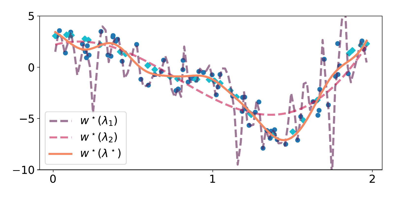
Figure 11.1: Hyperparameter optimization in nonlinear regression can be cast as a bi-level optimization problem. Each line corresponds to the estimator obtained by fitting some training data (in blue circles) using a different hyperparameter $λ$ λ. Formally, denoting $f$ f the training objective, the estimators are $w^{⋆} (λ) ≔ {arg min}_{w} f (w; λ)$ w⋆(λ):=argminwf(w;λ). The goal is to find the best hyperparameter that fits some validation data (here in cyan diamonds), that is, minimizing $h (λ) ≔ g (w^{⋆} (λ), λ)$ h(λ):=g(w⋆(λ),λ), where $g$ g is the validation objective. A too small $λ_{1}$ λ1 leads to overfitting the training objective and performs badly on validation objective. Conversely, a larger $λ_{2}$ λ2 underfits both training and validation objectives. The optimal parameter $λ^{⋆}$ λ⋆ minimizes the validation objective and may be obtained by iterating gradient descent w.r.t. $λ$ λ. This requires gradients of $h (λ) = g (w^{⋆} (λ), λ)$ h(λ)=g(w⋆(λ),λ) w.r.t. $λ$ λ.

11.2 Envelope theorems

In the special case $g = f$ g=f, the composition $h$ h defined in Eq. (11.1) is simply given by $h (λ) = f (w^{⋆} (λ), λ) = \max_{w \in W} f (w, λ) .$ h(λ)=f(w⋆(λ),λ)=w∈Wmaxf(w,λ). That is, we no longer need argmax differentiation, but only max differentiation, which, as we shall now see is much easier. The function $h$ h is often called a value function (Fleming and Rishel, 2012). The reason for the name “envelope” is illustrated in Fig. 11.2. We emphasize that there is not one, but several envelope theorems, depending on the assumptions on $f$ f.

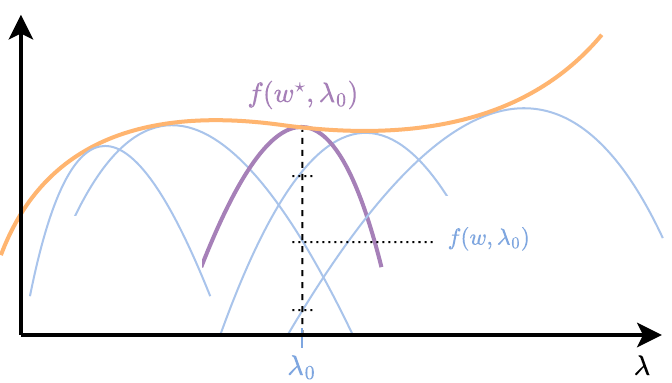
Figure 11.2: The graph of $h (λ) = \max_{w \in W} f (w, λ)$ h(λ)=maxw∈Wf(w,λ) is the upper-envelope of the graphs of the functions $λ \mapsto f (w, λ)$ λ↦f(w,λ) for all $w \in W$ w∈W.

11.2.1 Bertsekas’ theorem

The following theorem is due to Bertsekas (1997, Proposition B.25).

Theorem 11.1 (Bertsekas’ theorem)

Let $h (λ) ≔ \max_{w \in W} f (w, λ)$ h(λ):=w∈Wmaxf(w,λ) and $w^{⋆} (λ) ≔ \underset{w \in W}{arg max} f (w, λ),$ w⋆(λ):=w∈Wargmaxf(w,λ), where $f ⁣ : W \times Λ \to R$ f:W×Λ→R is concave in $w$ w and $W$ W is a compact convex set. If the maximum $w^{⋆} (λ)$ w⋆(λ) is unique, then the function $h$ h is differentiable with gradient $\nabla h (λ) = \nabla_{2} f (w^{⋆} (λ), λ) .$ ∇h(λ)=∇2f(w⋆(λ),λ). If furthermore $f$ f is convex in $λ$ λ, then $h (λ)$ h(λ) is convex.

A variant of the theorem can be stated when $W = R^{P}$ W=RP.

Theorem 11.2 (Unbounded case)

Suppose $W = R^{P}$ W=RP. If $f$ f is strongly concave in $w$ w, then the function $h$ h is differentiable with gradient $\nabla h (λ) = \nabla_{2} f (w^{⋆} (λ), λ) .$ ∇h(λ)=∇2f(w⋆(λ),λ). If furthermore $f$ f is convex in $λ$ λ, then $h (λ)$ h(λ) is convex.

Informally, Theorem 11.1 and Theorem 11.2 mean that we can treat $w^{⋆} (λ)$ w⋆(λ) as if it were a constant of $λ$ λ. In other words, we do not need to differentiate through $w^{⋆} (λ)$ w⋆(λ), even though it depends on $λ$ λ.

Remark 11.1 (Historical note)

Bertsekas’ theorem or its unbounded variant are often incorrectly cited as Danskin’s theorem in the machine learning literature, because Bertsekas himself called it that way (Bertsekas, 1997, Proposition B.25). However, because the assumptions differ, they should rather be thought as variants or corollaries of Danskin’s original theorem. See Section 11.2.3 for more details.

We now illustrate Theorem 11.2, to differentiate through a minimum, $h (λ) = \min_{w \in W} f (w, λ)$ h(λ)=minw∈Wf(w,λ), assuming $f (w, λ)$ f(w,λ) is strongly convex in $w$ w.

Example 11.1 (Differentiating the minimum of a convex quadratic)

Let us define $h (λ) ≔ \min_{w \in R} f (w, λ)$ h(λ):=minw∈Rf(w,λ), where $f (w, λ) ≔ \frac{λ}{2} w^{2} + b w + c$ f(w,λ):=2λw2+bw+c and $λ > 0$ λ>0. The derivative of $f$ f w.r.t. $w$ w is $\nabla_{1} f (w, λ) = λ w + b$ ∇1f(w,λ)=λw+b. The second derivative of $f$ f w.r.t. $w$ w is $\nabla_{1}^{2} f (w, λ) = λ$ ∇12f(w,λ)=λ. Therefore $f$ f is strongly convex in $w$ w. Let $w^{⋆} (λ)$ w⋆(λ) be the minimum of $f$ f in $w$ w. Setting $\nabla_{1} f (w, λ)$ ∇1f(w,λ) to zero, we get $w^{⋆} (λ) = - \frac{b}{λ}$ w⋆(λ)=−λb. The derivative of $f$ f w.r.t. $λ$ λ is $\nabla_{2} f (w, λ) = \frac{1}{2} w^{2}$ ∇2f(w,λ)=21w2. From Theorem 11.2, we have $h^{'} (λ) = \nabla_{2} f (w^{⋆} (λ), λ) = \frac{1}{2} (w^{⋆} (λ))^{2} = \frac{1}{2} \frac{b^{2}}{λ^{2}}$ h′(λ)=∇2f(w⋆(λ),λ)=21(w⋆(λ))2=21λ2b2. Let us check that the derivative is indeed correct. Plugging $w^{⋆} (λ)$ w⋆(λ) back into $f (w, λ)$ f(w,λ), we get the analytical formula $h (λ) = - \frac{1}{2} \frac{b^{2}}{λ} + c$ h(λ)=−21λb2+c. Using $(\frac{1}{λ})^{'} = - \frac{1}{λ^{2}}$ (λ1)′=−λ21, we indeed obtain the same expression for $h^{'} (λ)$ h′(λ).

Theorem 11.1 has a simple interpretation for functions that are affine in $λ$ λ as shown below.

Example 11.2 (Convex conjugate)

Let $f (w, λ) ≔ ⟨ w, λ ⟩ - Ω (w)$ f(w,λ):=⟨w,λ⟩−Ω(w) with $Ω$ Ω convex. We then have $h (λ) = \max_{w \in W} ⟨ w, λ ⟩ - Ω (w) ≕ Ω^{*} (λ)$ h(λ)=maxw∈W ⟨w,λ⟩−Ω(w)=:Ω∗(λ), where $Ω^{*}$ Ω∗ denotes the convex conjugate of $Ω$ Ω. Since $f$ f is convex and assuming $W$ W is convex compact, the conditions of Theorem 11.1 are met. Since $\nabla_{2} f (w, λ) = w$ ∇2f(w,λ)=w, we obtain $\nabla h (λ) = \nabla Ω^{*} (λ) = w^{⋆} (λ)$ ∇h(λ)=∇Ω∗(λ)=w⋆(λ). In other words, in this special case, the gradient of the max is equal to the argmax. This is due to the fact that $f (w, λ)$ f(w,λ) is affine in $λ$ λ.

Another application is saddle point optimization.

Example 11.3 (Saddle point problem)

Consider the saddle point problem $\min_{λ \in Λ} \max_{w \in W} f (w, λ)$ minλ∈Λmaxw∈Wf(w,λ). If it is difficult to minimize w.r.t. $λ$ λ but easy to maximize w.r.t. $w$ w, we can rewrite the problem as $\min_{λ \in Λ} h (λ)$ minλ∈Λh(λ), where $h (λ) ≔ \max_{w \in W} f (w, λ)$ h(λ):=maxw∈Wf(w,λ), and use $\nabla h (λ)$ ∇h(λ) to perform (projected) gradient descent w.r.t. $λ$ λ.

11.2.2 Rockafellar’s theorem

A related theorem (Rockafellar and Wets, 2009, Theorem 10.31) can be proved under different assumptions on $f$ f.

Theorem 11.3 (Rockafellar’s envelope theorem)

Let $f ⁣ : W \times Λ \to R$ f:W×Λ→R and $W$ W be a compact convex set. Let $h (λ) ≔ \max_{w \in W} f (w, λ)$ h(λ):=w∈Wmaxf(w,λ) and $w^{⋆} (λ) ≔ \underset{w \in W}{arg max} f (w, λ) .$ w⋆(λ):=w∈Wargmaxf(w,λ). If $f$ f is continuously differentiable in $λ$ λ for all $w \in W$ w∈W, $\nabla_{1} f$ ∇1f is continuous and the maximum $w^{⋆} (λ)$ w⋆(λ) is unique, then the function $h$ h is differentiable with gradient $\nabla h (λ) = \nabla_{2} f (w^{⋆} (λ), λ) .$ ∇h(λ)=∇2f(w⋆(λ),λ).

Compared to Bertsekas’ theorem, Rockafellar’s theorem does not require $f$ f to be concave in $w$ w, but it requires stronger assumptions on the differentiability of $f$ f.

11.2.3 Danskin’s theorem

Finally, we state Danskin’s original theorem (Danskin, 1966).

Theorem 11.4 (Danskin’s theorem)

Let $W$ W be a compact topological space. Let $f ⁣ : W \times Λ \to R$ f:W×Λ→R be continuous and continuously differentiable with respect to $λ \in Λ$ λ∈Λ. Let the value function and the set of maximizers be defined as $h (λ) ≔ \max_{w \in W} f (w, λ) and W^{⋆} (λ) ≔ \underset{w \in W}{arg max} f (w, λ) .$ h(λ):=w∈Wmaxf(w,λ)andW⋆(λ):=w∈Wargmaxf(w,λ). Then, the directional derivative of $h$ h at $λ \in Λ$ λ∈Λ in direction $d \in Λ$ d∈Λ, denoted $h^{'} (λ; d)$ h′(λ;d), exists and is given by $h^{'} (λ; d) = \max_{w \in W^{⋆} (λ)} ⟨ \nabla_{2} f (w, λ), d ⟩ .$ h′(λ;d)=w∈W⋆(λ)max⟨∇2f(w,λ),d⟩.

We sum up envelope theorems and their assumptions in Table 11.1.

Table 11.1: Comparison of different envelope theorems.

Theorem	Unique $w^{⋆}$ w⋆?	Concave in $w$ w?	Smooth in $w$ w?	Result
Danskin	No	No	No	Dir. Deriv.
Bertsekas	Yes	Yes	No	Gradient
Rockafellar	Yes	No	Yes	Gradient

11.3 Implicit function theorem

11.3.1 Univariate functions

The implicit function theorem (IFT) provides conditions under which an implicit relationship of the form $F (w, λ) = 0$ F(w,λ)=0 can be rewritten as a function $w = w^{⋆} (λ)$ w=w⋆(λ) locally, and provides a way to compute its derivative w.r.t. $λ$ λ.

Theorem 11.5 (Implicit function theorem, univariate case)

Let
$F ⁣ : R \times R \to R$ F:R×R→R. Assume $F (w, λ)$ F(w,λ) is a continuously differentiable function in a neighborhood $U$ U of $(w_{0}, λ_{0})$ (w0,λ0) such that $F (w_{0}, λ_{0}) = 0$ F(w0,λ0)=0 and $\partial_{1} F (w_{0}, λ_{0}) \neq 0$ ∂1F(w0,λ0)=0. Then there exists a neighborhood $V \subseteq U$ V⊆U of $(w_{0}, λ_{0})$ (w0,λ0) in which there is a function $w^{⋆} (λ)$ w⋆(λ) such that

$w^{⋆} (λ_{0}) = w_{0}$ w⋆(λ0)=w0,
$F (w^{⋆} (λ), λ) = 0$ F(w⋆(λ),λ)=0 for all $λ$ λ in the neighborhood $V$ V,
$\partial w^{⋆} (λ) = - \frac{\partial_{2} F (w^{⋆} (λ), λ)}{\partial_{1} F (w^{⋆} (λ), λ)}$ ∂w⋆(λ)=−∂1F(w⋆(λ),λ)∂2F(w⋆(λ),λ).

We postpone the proof to the multivariate case and begin with a classical example of application of the theorem.

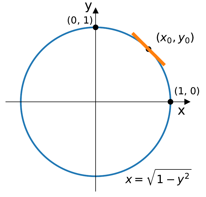
Figure 11.3: The circle equation $F (x, y) ≔ x^{2} + y^{2} - 1 = 0$ F(x,y):=x2+y2−1=0 is not a function from $y \in [- 1, 1]$ y∈[−1,1] to $x \in [- 1, 1]$ x∈[−1,1], as there are always two possible $x$ x values, $x = \sqrt{1 - y^{2}}$ x=1−y2 or $x = - \sqrt{1 - y^{2}}$ x=−1−y2. However, locally around some point $(x_{0}, y_{0})$ (x0,y0), e.g., such that $x_{0} > 0$ x0>0 and $y_{0} > 0$ y0>0 (upper-right quadrant), the function $x = x^{⋆} (y) = \sqrt{1 - y^{2}}$ x=x⋆(y)=1−y2 is well-defined. The implicit function theorem gives conditions for such a function to exist locally and provides a way to compute its derivative.

Example 11.4 (Equation of the unit circle)

We use $w \equiv x$ w≡x and $λ \equiv y$ λ≡y for clarity. Let $F (x, y) ≔ x^{2} + y^{2} - 1$ F(x,y):=x2+y2−1. In general, we cannot rewrite the unit circle equation $F (x, y) = 0$ F(x,y)=0 as a function from $y$ y to $x$ x, because for every $y \in [- 1, 1]$ y∈[−1,1], there are always two possible $x$ x values, namely, $x = \sqrt{1 - y^{2}}$ x=1−y2 or $x = - \sqrt{1 - y^{2}}$ x=−1−y2. However, locally around some point $(x_{0}, y_{0})$ (x0,y0), e.g., such that $x_{0} > 0$ x0>0 and $y_{0} > 0$ y0>0 (upper-right quadrant), the function $x = x^{⋆} (y) = \sqrt{1 - y^{2}}$ x=x⋆(y)=1−y2 is well-defined. Using $\partial_{1} F (x, y) = 2 x$ ∂1F(x,y)=2x and $\partial_{2} F (x, y) = 2 y$ ∂2F(x,y)=2y, we get $\partial x^{⋆} (y) = - \frac{\partial_{2} F (x^{⋆} (y), y)}{\partial_{1} F (x^{⋆} (y), y)} = - \frac{2 y}{2 x^{⋆} (y)} = - \frac{y}{\sqrt{1 - y^{2}}}$ ∂x⋆(y)=−∂1F(x⋆(y),y)∂2F(x⋆(y),y)=−2x⋆(y)2y=−1−y2y in that neighborhood (the upper right quadrant in this case). This is indeed the same derivative expression as if we used the chain rule on $\sqrt{1 - y^{2}}$ 1−y2 and is well-defined on $y \in [0, 1)$ y∈[0,1).

In the above simple example, we can easily derive an explicit function relating $y$ y to $x$ x in a given neighborhood, but this is not always the case. The IFT gives us conditions guaranteeing that such function exists and a way to differentiate it, but not a way to construct such a function. In fact, finding $w^{⋆} (λ)$ w⋆(λ) such that $F (w^{⋆} (λ), λ) = 0$ F(w⋆(λ),λ)=0 typically involves a root finding algorithm, an optimization algorithm, a nonlinear system solver, etc.

Example 11.5 (Polynomial)

Let $F (w, λ) = w^{5} + w^{3} + w - λ$ F(w,λ)=w5+w3+w−λ. According to the Abel-Ruffini theorem (Tignol, 2015), quintics (polynomials of degree $5$ 5) do not enjoy roots in terms of radicals and one must resort to numerical root finding. In addition, odd-degree polynomials have real roots. Moreover, $\partial_{1} F (w, λ) = 5 w^{4} + 3 w^{2} + 1$ ∂1F(w,λ)=5w4+3w2+1 is strictly positive. Therefore, by the intermediate value theorem, there must be only one root $w^{⋆} (λ)$ w⋆(λ) such that $F (w^{⋆} (λ), λ) = 0$ F(w⋆(λ),λ)=0. This unique root can for example be found by bisection. Using the IFT, its derivative is found to be $\partial w^{⋆} (λ) = (5 w^{⋆} (λ)^{4} + 3 w^{⋆} (λ)^{2} + 1)^{- 1}$ ∂w⋆(λ)=(5w⋆(λ)4+3w⋆(λ)2+1)−1.

While an implicit function is differentiable at a point if the assumptions of the IFT hold in a neighborhood of that point, the reciprocal is not true: failure of the IFT assumptions does not necessarily mean that the implicit function is not differentiable, as we now illustrate.

Example 11.6 (IFT conditions are not necessary for differentiability)

Consider $F (w, λ) = (w - λ)^{2}$ F(w,λ)=(w−λ)2. We clearly have that $F (w^{⋆} (λ), λ) = 0$ F(w⋆(λ),λ)=0 if we define $w^{⋆} (λ) = λ$ w⋆(λ)=λ, the identity function. It is clearly differentiable for all $λ$ λ, yet the assumptions of the IFT fail, since we have $\partial_{1} F (w, λ) = 2 (w - λ)$ ∂1F(w,λ)=2(w−λ) and therefore $\partial_{1} F (0, 0) = 0$ ∂1F(0,0)=0.

11.3.2 Multivariate functions

We now present the IFT in the general multivariate setting. Informally, if $F (w^{⋆} (λ), λ) = 0$ F(w⋆(λ),λ)=0, then by the chain rule, we have $\partial_{1} F (w^{⋆} (λ), λ) \partial w^{⋆} (λ) + \partial_{2} F (w^{⋆} (λ), λ) = 0,$ ∂1F(w⋆(λ),λ)∂w⋆(λ)+∂2F(w⋆(λ),λ)=0, meaning that the Jacobian $\partial w^{⋆} (λ)$ ∂w⋆(λ), assuming that it exists, satisfies $- \partial_{1} F (w^{⋆} (λ), λ) \partial w^{⋆} (λ) = \partial_{2} F (w^{⋆} (λ), λ) .$ −∂1F(w⋆(λ),λ)∂w⋆(λ)=∂2F(w⋆(λ),λ). The IFT gives us conditions for the existence of $\partial w^{⋆} (λ)$ ∂w⋆(λ).

Theorem 11.6 (Implicit function theorem, multivariate case)

Let us define $F ⁣ : W \times Λ \to W$ F:W×Λ→W. Assume $F (w, λ)$ F(w,λ) is a continuously differentiable function in a neighborhood of $(w_{0}, λ_{0})$ (w0,λ0) such that $F (w_{0}, λ_{0}) = 0$ F(w0,λ0)=0 and $\partial_{1} F (w_{0}, λ_{0})$ ∂1F(w0,λ0) is invertible, i.e., its determinant is nonzero. Then there exists a neighborhood of $λ_{0}$ λ0 in which there is a function $w^{⋆} (λ)$ w⋆(λ) such that

$w^{⋆} (λ_{0}) = w_{0}$ w⋆(λ0)=w0,
$F (w^{⋆} (λ), λ) = 0$ F(w⋆(λ),λ)=0 for all $λ$ λ in the neighborhood,
$- \partial_{1} F (w^{⋆} (λ), λ) \partial w^{⋆} (λ) = \partial_{2} F (w^{⋆} (λ), λ)$ −∂1F(w⋆(λ),λ)∂w⋆(λ)=∂2F(w⋆(λ),λ)

$⟺ \partial w^{⋆} (λ) = - \partial_{1} F (w^{⋆} (λ), λ)^{- 1} \partial_{2} F (w^{⋆} (λ), λ) .$ ⟺∂w⋆(λ)=−∂1F(w⋆(λ),λ)−1∂2F(w⋆(λ),λ).

We begin with a simple unconstrained optimization algorithm.

Example 11.7 (Unconstrained optimization)

Assume we want to differentiate through $w^{⋆} (λ) = {arg min}_{w \in R^{P}} f (w, λ)$ w⋆(λ)=argminw∈RPf(w,λ), where $f$ f is strictly convex in $w$ w, which ensures that the solution is unique. From the stationary conditions, if we define $F (w, λ) ≔ \nabla_{1} f (w, λ)$ F(w,λ):=∇1f(w,λ), then $w^{⋆} (λ)$ w⋆(λ) is uniquely characterized as the root of $F$ F in the first argument, i.e., $F (w^{⋆} (λ), λ) = 0$ F(w⋆(λ),λ)=0. We have $\partial_{1} F (w, λ) = \nabla_{1}^{2} f (w, λ)$ ∂1F(w,λ)=∇12f(w,λ), the Hessian of $f$ f in $w$ w, and $\partial_{2} F (w, λ) = \partial_{2} \nabla_{1} f (w, λ)$ ∂2F(w,λ)=∂2∇1f(w,λ), the cross derivatives of $f$ f in $w$ w and $λ$ λ. Therefore, assuming that the Hessian is well-defined and invertible at $(w^{⋆} (λ), λ)$ (w⋆(λ),λ), we can use the IFT to differentiate through $w^{⋆} (λ)$ w⋆(λ) and obtain $\partial w^{⋆} (λ) = - (\nabla_{1}^{2} f (w^{⋆} (λ), λ))^{- 1} \partial_{2} \nabla_{1} f (w^{⋆} (λ), λ)$ ∂w⋆(λ)=−(∇12f(w⋆(λ),λ))−1∂2∇1f(w⋆(λ),λ).

Next, we generalize the previous example, by allowing constraints in the optimization problem.

Example 11.8 (Constrained optimization)

Now, assume we want to differentiate through $w^{⋆} (λ) = {arg min}_{w \in C} f (w, λ)$ w⋆(λ)=argminw∈Cf(w,λ), where $f$ f is strictly convex in $w$ w and $C \subseteq W$ C⊆W is a convex set. A solution is characterized by the fixed point equation $w^{⋆} (λ) = P_{C} (w^{⋆} (λ) - η \nabla_{1} f (w^{⋆} (λ), λ))$ w⋆(λ)=PC(w⋆(λ)−η∇1f(w⋆(λ),λ)), for any $η > 0$ η>0, where $P (y) ≔ {arg min}_{x \in C} ∥ x - y ∥_{2}^{2}$ P(y):=argminx∈C∥x−y∥22 is the Euclidean projection of $y$ y onto $C$ C. Therefore, $w^{⋆} (λ)$ w⋆(λ) is the root of $F (w, λ) = w - P_{C} (w - η \nabla_{1} f (w, λ))$ F(w,λ)=w−PC(w−η∇1f(w,λ)) (see Chapter 16). We can differentiate through $w^{⋆} (λ)$ w⋆(λ) using the IFT, assuming that the conditions of the theorem apply. Note that $\partial_{1} F (w, λ)$ ∂1F(w,λ) requires the expression of the Jacobian $\partial P_{C} (y)$ ∂PC(y). Fortunately, $P_{C} (y)$ PC(y) and its Jacobian are easy to compute for many sets $C$ C (Blondel et al., 2021).

11.3.3 JVP and VJP of implicit functions

To integrate an implicit function $w^{⋆} (λ)$ w⋆(λ) in an autodiff framework, we need to be able to compute its JVP or VJP. This is the purpose of the next proposition.

Proposition 11.1 (JVP and VJP of implicit functions)

Let $w^{⋆} ⁣ : Λ \to W$ w⋆:Λ→W be a function implicitly defined as the solution of $F (w^{⋆} (λ), λ) = 0$ F(w⋆(λ),λ)=0, for some function $F ⁣ : W \times Λ \to W$ F:W×Λ→W. Define $\begin{matrix} A & ≔ - \partial_{1} F (w^{⋆} (λ), λ) \\ B & ≔ \partial_{2} F (w^{⋆} (λ), λ) . \end{matrix}$ AB:=−∂1F(w⋆(λ),λ):=∂2F(w⋆(λ),λ). Assume the assumptions of the IFT hold. The JVP $t ≔ \partial w^{⋆} (λ) v$ t:=∂w⋆(λ)v in the input direction $v \in Λ$ v∈Λ is obtained by solving the linear system $A t = B v .$ At=Bv. The VJP $\partial w^{⋆} (λ)^{*} u$ ∂w⋆(λ)∗u in the output direction $u \in W$ u∈W is obtained by solving the linear system $A^{*} r = u .$ A∗r=u. Using the solution $r$ r, we get $\partial w^{⋆} (λ)^{*} u = \partial w^{⋆} (λ)^{*} A^{*} r = B^{*} r .$ ∂w⋆(λ)∗u=∂w⋆(λ)∗A∗r=B∗r.

Note that in the above linear systems, we can access $A$ A and $B$ B as linear maps, the JVPs of $F$ F. Their adjoints, $A^{*}$ A∗ and $B^{*}$ B∗, correspond to the VJPs of $F$ F. To solve these systems, we can therefore use matrix-free solvers as detailed in Section 9.4. For example, when $A$ A is symmetric positive semi-definite, we can use the conjugate gradient method (Hestenes et al., 1952). When $A$ A is not symmetric positive definite, we can use GMRES (Saad and Schultz, 1986) or BiCGSTAB (Vorst and Vorst, 1992).

11.3.4 Proof of the implicit function theorem

We prove the theorem using the inverse function theorem presented in Theorem 11.7. Define $f (λ, w) = (λ, F (w, λ))$ f(λ,w)=(λ,F(w,λ)) which goes from $R^{Q} \times R^{P}$ RQ×RP onto $R^{Q} \times R^{P}$ RQ×RP. The Jacobian of $f$ f is $\partial f (λ, w) = (\begin{matrix} I & 0 \\ \partial_{2} F (w, λ) & \partial_{1} F (w, λ) \end{matrix}) .$ ∂f(λ,w)=(I∂2F(w,λ)0∂1F(w,λ)). So at $w_{0}, λ_{0}$ w0,λ0, we have $\det (\partial f (λ_{0}, w_{0})) = \det (I) \det (\partial_{1} F (w_{0}, λ_{0})) \neq 0$ det(∂f(λ0,w0))=det(I)det(∂1F(w0,λ0))=0 since we assumed $\partial_{1} F (w_{0}, λ_{0})$ ∂1F(w0,λ0) invertible. By the inverse function theorem, the function $f$ f is then invertible in a neighborhood $N$ N of $f (λ_{0}, w_{0}) = (λ_{0}, 0)$ f(λ0,w0)=(λ0,0). In particular, it is invertible in $N \cap {(λ, 0), λ \in R^{Q}}$ N∩{(λ,0),λ∈RQ}. The solution of the implicit equation in a neighborhood of $λ_{0}$ λ0 is then $(λ, w^{*} (λ)) = f^{- 1} (λ, 0)$ (λ,w∗(λ))=f−1(λ,0). By the inverse function theorem, $f^{- 1}$ f−1 is continuously differentiable inverse and so is $w^{*} (λ)$ w∗(λ). The derivative $\partial w^{*} (λ)$ ∂w∗(λ) is obtained from the differential of the inverse as $(\begin{matrix} \sim & \sim \\ \partial w^{*} (λ) & \sim \end{matrix}) = \partial f^{- 1} (λ, 0),$ (∼∂w∗(λ)∼∼)=∂f−1(λ,0), and by the inverse function theorem, we have $\partial f^{- 1} (λ, 0) = (\partial f (λ, w^{*} (λ)))^{- 1} .$ ∂f−1(λ,0)=(∂f(λ,w∗(λ)))−1. Using the block matrix inversion formula, we therefore obtain ${(\begin{matrix} A & B \\ C & D \end{matrix})}^{- 1} = (\begin{matrix} \sim & \sim \\ - (D - C A^{- 1} B)^{- 1} C A^{- 1} & \sim \end{matrix}),$ (ACBD)−1=(∼−(D−CA−1B)−1CA−1∼∼), we get the claimed expression. Though we expressed the proof in terms of Jacobians and matrices, the result naturally holds for the corresponding linear operators, JVPs, VJPs, and their inverses.

11.4 Adjoint state method

11.4.1 Differentiating nonlinear equations

We describe in this section the adjoint state method (a.k.a. adjoint method, method of adjoints, adjoint sensitivity method). The method can be used to compute the gradient of the composition of an explicit function and an implicit function, defined through an equality constraint (e.g., a nonlinear equation). The method dates back to Céa (1986).

Suppose a variable $s \in S$ s∈S (which corresponds to a state in optimal control) is implicitly defined given some parameters $w \in W$ w∈W through the (potentially nonlinear) equation $c (s, w) = 0$ c(s,w)=0, where $c ⁣ : S \times W \to S$ c:S×W→S. Assuming $s$ s is uniquely determined for all $w \in W$ w∈W, this defines an implicit function $s^{⋆} (w)$ s⋆(w) from $W$ W to $S$ S such that $c (s^{⋆} (w), w) = 0$ c(s⋆(w),w)=0. Given an objective function $L ⁣ : S \times W \to R$ L:S×W→R, the goal of the adjoint state method is then to compute the gradient of $L (w) ≔ L (s^{⋆} (w), w) .$ L(w):=L(s⋆(w),w). However, this is not trivial as $s^{⋆} (w)$ s⋆(w) is an implicit function. For instance, this can be used to convert the equality-constrained problem $\begin{matrix} \min_{w \in W} L (s, w) s.t. c (s, w) = 0. \end{matrix}$ w∈WminL(s,w)s.t.c(s,w)=0. into the unconstrained problem $\begin{matrix} \min_{w \in W} L (s^{⋆} (w), w) . \end{matrix}$ w∈WminL(s⋆(w),w). Access to $\nabla L (w)$ ∇L(w) allows us to solve this problem by gradient descent.

Proposition 11.2 (Adjoint state method)

Let $c : S \times W \to S$ c:S×W→S be a mapping defining constraints of the form $c (s, w)$ c(s,w). Assume that for each $w \in W$ w∈W, there exists a unique $s^{⋆} (w)$ s⋆(w) satisfying $c (s^{⋆} (w), w) = 0$ c(s⋆(w),w)=0 and that $s^{⋆} (w)$ s⋆(w) is differentiable. The gradient of $L (w) ≔ L (s^{⋆} (w), w),$ L(w):=L(s⋆(w),w), for some differentiable function $L : S \times W \to R$ L:S×W→R, is given by $\nabla L (w) = \nabla_{2} L (s^{⋆} (w), w) + \partial_{2} c (s^{⋆} (w), w)^{*} r^{⋆} (w),$ ∇L(w)=∇2L(s⋆(w),w)+∂2c(s⋆(w),w)∗r⋆(w), where $r^{⋆} (w)$ r⋆(w) is the solution of the linear system $\partial_{1} c (s^{⋆} (w), w)^{*} r = - \nabla_{1} L (s^{⋆} (w), w) .$ ∂1c(s⋆(w),w)∗r=−∇1L(s⋆(w),w).

As shown in the proof below, $r^{⋆} (w)$ r⋆(w) corresponds to a Lagrange multiplier. The linear system can be solved using matrix-free solvers.

11.4.2 Relation with envelope theorems

Because $s$ s is uniquely determined for any $w \in W$ w∈W by $c (s, w) = 0$ c(s,w)=0, we can alternatively rewrite $L (w)$ L(w) as the trivial minimization or maximization, $\begin{matrix} L (w) & = \min_{s \in S} L (s, w) s.t. c (s, w) = 0 \\ = \max_{s \in S} L (s, w) s.t. c (s, w) = 0. \end{matrix}$ L(w)=s∈SminL(s,w)s.t.c(s,w)=0=s∈SmaxL(s,w)s.t.c(s,w)=0. Therefore, the adjoint state method can be seen as an envelope theorem for computing $\nabla L (w)$ ∇L(w), for the case when $w$ w is involved in both the objective function and in the equality constraint.

11.4.3 Proof using the method of Lagrange multipliers

Classically, the adjoint state method is derived using the method of Lagrange multipliers. Let us introduce the Lagrangian associated with $L$ L and $c$ c, $L (s, w, r) ≔ L (s, w) + ⟨ r, c (s, w) ⟩,$ L(s,w,r):=L(s,w)+⟨r,c(s,w)⟩, where $r \in S$ r∈S is the Lagrange multiplier associated with the equality constraint $c (s, w) = 0$ c(s,w)=0. In the optimal control literature, $r$ r is often called the adjoint variable or adjoint state. The gradients of the Lagrangian are $\begin{matrix} \nabla_{s} L (s, w, r) & = \nabla_{1} L (s, w) + \partial_{1} c (s, w)^{*} r \\ \nabla_{w} L (s, w, r) & = \nabla_{2} L (s, w) + \partial_{2} c (s, w)^{*} r \\ \nabla_{r} L (s, w, r) & = c (s, w), \end{matrix}$ ∇sL(s,w,r)∇wL(s,w,r)∇rL(s,w,r)=∇1L(s,w)+∂1c(s,w)∗r=∇2L(s,w)+∂2c(s,w)∗r=c(s,w), where $\partial_{i} c (s, w)^{*}$ ∂ic(s,w)∗ are the adjoint operators. Setting $\nabla_{r} L (s, w, r)$ ∇rL(s,w,r) to zero gives the constraint $c (s, w) = 0$ c(s,w)=0. Setting $\nabla_{s} L (s, w, r)$ ∇sL(s,w,r) to zero gives the so-called adjoint state equation $\partial_{1} c (s, w)^{*} r = - \nabla_{1} L (s, w) .$ ∂1c(s,w)∗r=−∇1L(s,w). Solving this linear system w.r.t. $r$ r at $s = s^{⋆} (w)$ s=s⋆(w) gives the adjoint variable $r^{⋆} (w)$ r⋆(w). We then get $\begin{matrix} \nabla L (w) & = \nabla_{2} L (s^{⋆} (w), w, r^{⋆} (w)) \\ = \nabla_{2} L (s^{⋆} (w), w) + \partial_{2} c (s^{⋆} (w), w)^{*} r^{⋆} (w), \end{matrix}$ ∇L(w)=∇2L(s⋆(w),w,r⋆(w))=∇2L(s⋆(w),w)+∂2c(s⋆(w),w)∗r⋆(w), which concludes the proof.

11.4.4 Proof using the implicit function theorem

A more direct proof is possible thanks to the implicit function theorem (Section 11.3). Using the chain rule, we get $\nabla L (w) = \nabla_{2} L (s^{⋆} (w), w) + \partial s^{⋆} (w)^{*} \nabla_{1} L (s^{⋆} (w), w),$ ∇L(w)=∇2L(s⋆(w),w)+∂s⋆(w)∗∇1L(s⋆(w),w), where $\partial s^{⋆} (w)^{*}$ ∂s⋆(w)∗ is the VJP of $s^{⋆}$ s⋆, a linear map from $S$ S to $W$ W.

Computationally, the main difficulty is to apply $\partial s^{⋆} (w)^{*}$ ∂s⋆(w)∗ to the vector $u = \nabla_{1} L (s^{⋆} (w), w) \in S$ u=∇1L(s⋆(w),w)∈S. Using the implicit function theorem (Section 11.3) on the implicit function $c (s^{⋆} (w), w) = 0$ c(s⋆(w),w)=0, and Proposition 11.1, we get the linear system $A^{*} r = u$ A∗r=u, where $A^{*} ≔ \partial_{1} c (s^{⋆} (w), w)^{*}$ A∗:=∂1c(s⋆(w),w)∗ is a linear map from $S$ S to $S$ S. After solving for $r$ r, we get $\partial s^{⋆} (w)^{*} u = B^{*} r$ ∂s⋆(w)∗u=B∗r, where $B^{*} ≔ \partial_{2} c (s^{⋆} (w), w)^{*}$ B∗:=∂2c(s⋆(w),w)∗ is a linear map from $S$ S to $W$ W. Putting everything together, we get $\nabla L (w) = \nabla_{2} L (s^{⋆} (w), w) + \partial_{2} c (s^{⋆} (w), w)^{*} r .$ ∇L(w)=∇2L(s⋆(w),w)+∂2c(s⋆(w),w)∗r.

11.4.5 Reverse mode as adjoint method with backsubstitution

In this section, we revisit reverse-mode autodiff from the perspective of the adjoint state method. For clarity, we focus our exposition on feedforward networks with input $x \in X$ x∈X and network weights $w = (w_{1}, \dots, w_{k}) \in W_{1} \times \dots \times W_{K}$ w=(w1,…,wk)∈W1×…×WK, defined by $\begin{matrix} s_{0} & ≔ x \in X \\ s_{1} & ≔ f_{1} (s_{0}, w_{1}) \in S_{1} \\ ⋮ \\ s_{K} & ≔ f_{K} (s_{K - 1}, w_{K}) \in S_{K} \\ f (w) & ≔ s_{K} . \end{matrix}$ s0s1sKf(w):=x∈X:=f1(s0,w1)∈S1⋮:=fK(sK−1,wK)∈SK:=sK.(11.2) Here we focus on gradients with respect to the parameters $w$ w, hence the notation $f (w)$ f(w). We can use the adjoint state method to recover reverse-mode autodiff, and prove its correctness in the process. While we focus for simplicity on feedforward networks, our exposition can be generalized to computation graphs.

Feedforward networks as the solution of a nonlinear equation

While we defined the set of intermediate computations $s = (s_{1}, \dots, s_{K}) \in S_{1} \times \dots \times S_{K}$ s=(s1,…,sK)∈S1×…×SK as a sequence of operations, they can also be defined as the unique solution of the nonlinear equation $c (s, w) = 0$ c(s,w)=0, where $c (s, w) ≔ (\begin{matrix} s_{1} - f_{1} (x, w_{1}) \\ s_{2} - f_{2} (s_{1}, w_{2}) \\ ⋮ \\ s_{K} - f_{K} (s_{K - 1}, w_{K}) \end{matrix}) .$ c(s,w):=s1−f1(x,w1)s2−f2(s1,w2)⋮sK−fK(sK−1,wK). This defines an implicit function $s^{⋆} (w) = (s_{1}^{⋆} (w), \dots, s_{K}^{⋆} (w))$ s⋆(w)=(s1⋆(w),…,sK⋆(w)), the solution of this nonlinear system, which is given by the variables $s_{1}, \dots, s_{K}$ s1,…,sK defined in Eq. (11.2). The output of the feedforward network is then $f (w) = s_{K}^{⋆} (w)$ f(w)=sK⋆(w).

In machine learning, the final layer $s_{K}^{⋆} (w)$ sK⋆(w) is typically fed into a loss $ℓ$ ℓ, to define $L (w) ≔ ℓ (s_{K}^{⋆} (w); y) .$ L(w):=ℓ(sK⋆(w);y). Note that an alternative is to write $L (w)$ L(w) as $L (w) = \min_{s \in S} ℓ (s; y) s.t. c (s, w) = 0.$ L(w)=s∈Sminℓ(s;y)s.t.c(s,w)=0.

More generally, if we just want to compute the VJP of $s_{K}^{⋆} (w)$ sK⋆(w) in some direction $u_{K} \in S_{K}$ uK∈SK, we can define the scalar-valued function $L (w) ≔ ℓ (s_{K}^{⋆} (w); u_{K}) ≔ ⟨ s_{K}^{⋆} (w), u_{K} ⟩$ L(w):=ℓ(sK⋆(w);uK):=⟨sK⋆(w),uK⟩ so that $\partial f (w)^{*} u_{K} = \nabla L (w) .$ ∂f(w)∗uK=∇L(w). Let us define $u \in S_{1} \times \dots \times S_{K - 1} \times S_{K}$ u∈S1×⋯×SK−1×SK as $u ≔ (0, \dots, 0, \nabla_{1} ℓ (f (w); y))$ u:=(0,…,0,∇1ℓ(f(w);y)) (gradient of the loss $ℓ$ ℓ case) or $u ≔ (0, \dots, 0, u_{K})$ u:=(0,…,0,uK) (VJP of $f$ f in the direction $u_{K}$ uK case). Using the adjoint state method, we know that the gradient of this objective is obtained as $\nabla L (w) = \partial_{2} c (s (w), w)^{*} r^{⋆} (w),$ ∇L(w)=∂2c(s(w),w)∗r⋆(w), for $r^{⋆} (w)$ r⋆(w) the solution of the linear system $\partial_{1} c (s (w), w)^{*} r = - u .$ ∂1c(s(w),w)∗r=−u.

Solving the linear system using backsubtitution

The JVP of the constraint function $c$ c at $s^{⋆} (w)$ s⋆(w), materialized as a matrix, takes the form of a block lower-triangular matrix $\partial_{1} c (s^{⋆} (w), w) = (\begin{matrix} I & 0 & \dots & \dots & 0 \\ - A_{1} & I & ⋱ & ⋮ \\ 0 & - A_{2} & I & ⋱ & ⋮ \\ ⋮ & ⋱ & ⋱ & ⋱ & 0 \\ 0 & \dots & 0 & - A_{K} & I \end{matrix}),$ ∂1c(s⋆(w),w)=I−A10⋮00I−A2⋱……⋱I⋱0…⋱⋱−AK0⋮⋮0I, where $A_{k} ≔ \partial_{1} f_{k} (s_{k - 1}, w_{k})$ Ak:=∂1fk(sk−1,wk). Crucially the triangular structure of the JVP stems from the fact that each intermediate activation only depends on the past intermediate activations. Therefore, the constraints, corresponding to the lines of the Jacobian, cannot introduce non-zero values beyond its diagonal. The VJP takes the form of a block upper-triangular matrix $\partial_{1} c (s^{⋆} (w), w)^{*} = (\begin{matrix} I & - A_{1}^{*} & 0 & \dots & 0 \\ 0 & I & - A_{2}^{*} & ⋱ & ⋮ \\ ⋮ & ⋱ & I & ⋱ & 0 \\ ⋮ & ⋱ & ⋱ & - A_{K}^{*} \\ 0 & \dots & \dots & 0 & I \end{matrix}) .$ ∂1c(s⋆(w),w)∗=I0⋮⋮0−A1∗I⋱…0−A2∗I⋱……⋱⋱⋱00⋮0−AK∗I. Solving an upper triangular system like $\partial_{1} c (s (w), w)^{*} r = u$ ∂1c(s(w),w)∗r=u can then be done efficiently by backsubstitution. Starting from the last adjoint state $r_{K} = u$ rK=u, we can compute each adjoint state $r_{k}$ rk from that computed at $k + 1$ k+1. Namely, for $k \in (K - 1, \dots, 1)$ k∈(K−1,…,1), we have $\begin{matrix} r_{k} - A_{k + 1}^{*} r_{k + 1} = 0 ⟺ r_{k} = \partial f_{k + 1} (s_{k}, w_{k + 1})^{*} r_{k + 1} . \end{matrix}$ rk−Ak+1∗rk+1=0⟺rk=∂fk+1(sk,wk+1)∗rk+1. The VJPs with respect to the parameters are then obtained by $\partial_{2} c (s (w), w)^{*} r = (\begin{matrix} \partial_{2} f_{1} (x, w_{1})^{*} r_{1} \\ \partial_{2} f_{2} (s_{1} (w), w_{2})^{*} r_{2} \\ ⋮ \\ \partial_{2} f_{K} (s_{K - 1} (w), w_{K})^{*} r_{K} \end{matrix}),$ ∂2c(s(w),w)∗r=∂2f1(x,w1)∗r1∂2f2(s1(w),w2)∗r2⋮∂2fK(sK−1(w),wK)∗rK, recovering reverse-mode autodiff.

The Lagrangian perspective of backpropagation for networks with separate parameters $w = (w_{1}, \dots, w_{K})$ w=(w1,…,wK) is well-known; see for instance LeCun (1988) or Recht (2016). The Lagrangian perspective of backpropagation through time (Werbos, 1990) for networks with shared parameter $w$ w is discussed for instance by Franceschi et al. (2017). Our exposition uses the adjoint state method, which can itself be proved either using the method of Lagrange multipliers (Section 11.4.3) or by the implicit function theorem (Section 11.4.4), combined with backsubtitution for solving the upper-triangular linear system. Past works often minimize over $w$ w but we do not require this, as gradients are not necessarily used for optimization. Our exposition also supports computing the VJP of any vector-valued function $f$ f, while existing works derive the gradient of a scalar-valued loss function.

11.5 Inverse function theorem

11.5.1 Differentiating inverse functions

In some cases (see for instance Section 12.4.4), it is useful to compute the Jacobian of an inverse function $f^{- 1}$ f−1. The inverse function theorem below allows us to relate the Jacobian of $f^{- 1}$ f−1 with the Jacobian of $f$ f.

Theorem 11.7 (Inverse function theorem)

Assume $f ⁣ : W \to W$ f:W→W is continuously differentiable with invertible Jacobian $\partial f (w_{0})$ ∂f(w0) at $w_{0}$ w0. Then $f$ f is bijective from a neighborhood of $w_{0}$ w0 to a neighborhood of $f (w_{0})$ f(w0). Moreover, the inverse $f^{- 1}$ f−1 is continuously differentiable near $ω_{0} = f (w_{0})$ ω0=f(w0) and the Jacobian of the inverse $\partial f^{- 1} (ω)$ ∂f−1(ω) is $\partial f (w) \partial f^{- 1} (ω) = I \Leftrightarrow \partial f^{- 1} (ω) = (\partial f (w))^{- 1},$ ∂f(w)∂f−1(ω)=I⇔∂f−1(ω)=(∂f(w))−1, with $w = f^{- 1} (ω)$ w=f−1(ω).

11.5.2 Link with the implicit function theorem

The inverse function theorem can be used to prove the implicit function theorem; see proof of Theorem 11.6. Conversely, recall that, in order to use the implicit function theorem, we need to choose a root objective $F ⁣ : W \times Λ \to W$ F:W×Λ→W. If we set $W = Λ = R^{Q}$ W=Λ=RQ and $F (w, ω) = f (w) - ω$ F(w,ω)=f(w)−ω, with $f ⁣ : R^{Q} \to R^{Q}$ f:RQ→RQ, then we have that the root $w^{⋆} (ω)$ w⋆(ω) satisfying $F (w^{⋆} (ω), ω) = 0$ F(w⋆(ω),ω)=0 is exactly $w^{⋆} (ω) = f^{- 1} (ω)$ w⋆(ω)=f−1(ω). Moreover, $\partial_{1} F (w, ω) = \partial f (w)$ ∂1F(w,ω)=∂f(w) and $\partial_{2} F (w, ω) = - I$ ∂2F(w,ω)=−I. By applying the implicit function theorem with this $F$ F, we indeed recover the inverse function theorem.

11.5.3 Proof of inverse function theorem

We first give a proof of the formula assuming that $f^{- 1}$ f−1 is well-defined and continuously differentiable in a neighborhood of $f (w_{0})$ f(w0). In that case, we have for any $ω$ ω in a neighborhood of $f (w_{0})$ f(w0), $f \circ f^{- 1} (ω) = ω .$ f∘f−1(ω)=ω. Differentiating both sides w.r.t. $ω$ ω, we get $\partial f (f^{- 1} (ω)) \partial f^{- 1} (ω) = I,$ ∂f(f−1(ω))∂f−1(ω)=I, where $I$ I is the identity function in $R^{Q}$ RQ. In particular, for $w = f^{- 1} (ω)$ w=f−1(ω) we recover the formula presented in the statement.

Now, it remains to show that invertibility of the JVP ensures that the function is invertible in a neighborhood of $f (w_{0})$ f(w0) and that the inverse is continuously differentiable. For that, denote $l = \partial f (w_{0})$ l=∂f(w0) such that $l^{- 1}$ l−1 is well-defined by definition. $f$ f is invertible with continuously differentiable inverse, if and only if $l^{- 1} (f (w)) - f (w_{0})$ l−1(f(w))−f(w0) is invertible with continuously differentiable inverse. So without loss of generality, we consider $\partial f (w_{0}) = I$ ∂f(w0)=I, $f (w_{0}) = 0$ f(w0)=0, $w_{0} = 0$ w0=0.

As $f$ f is continuously differentiable, there exists a neighborhood $N ≔ {w : ∥ w - w_{0} ∥_{2} \leq δ}$ N:={w:∥w−w0∥2≤δ} on which we have $∥ \partial f (w) - I ∥_{2} \leq 1 / 2$ ∥∂f(w)−I∥2≤1/2. In this neighborhood, the function $g (w) = f (w) - w$ g(w)=f(w)−w is contractive by the mean value theorem with contraction factor $1 / 2$ 1/2. For any $ω$ ω such that $∥ ω - f (w_{0}) ∥_{2} \leq δ / 2$ ∥ω−f(w0)∥2≤δ/2, the sequence $w_{k + 1} = w_{k} - f (w_{k}) - ω^{'}$ wk+1=wk−f(wk)−ω′ remains in $N$ N and converges (since it is a Cauchy sequence by the contraction of $g$ g) to a unique fixed point $w_{\infty}$ w∞ satisfying $w_{\infty} = w_{\infty} - f (w_{\infty}) - ω ⟺ f (w_{\infty}) = ω$ w∞=w∞−f(w∞)−ω⟺f(w∞)=ω. This shows the existence of the inverse in the neighborhood $M ≔ {ω : ∥ ω - ω_{0} ∥_{2} \leq δ / 2}$ M:={ω:∥ω−ω0∥2≤δ/2} of $ω_{0} = f (w_{0})$ ω0=f(w0) onto $N$ N.

We tackle now the differentiability (hence the continuity) of $f^{- 1}$ f−1. For any $ω$ ω in the neighborhood of $ω_{0}$ ω0 with inverse $w ≔ f^{- 1} (ω) \in N$ w:=f−1(ω)∈N, the JVP of $f$ f at $w$ w satisfies by assumption $∥ \partial f (w) - I ∥_{2} \leq 1 / 2$ ∥∂f(w)−I∥2≤1/2. Hence, $a = \partial f (w) - I$ a=∂f(w)−I defines a convergent series $b = \sum_{k = 0}^{+ \infty} a^{k}$ b=∑k=0+∞ak and one verifies easily that $b = \partial f (w)^{- 1}$ b=∂f(w)−1, that is $\partial f (w)$ ∂f(w) is invertible and $∥ \partial f (w)^{- 1} ∥ \leq 2$ ∥∂f(w)−1∥≤2. To compute the JVP of the inverse, we consider then $\partial f (w)^{- 1}$ ∂f(w)−1 as the candidate JVP and examine $\frac{∥ f^{- 1} (ω + η) - f (ω) - (\partial f (w))^{- 1} η ∥_{2}}{∥ η ∥_{2}} .$ ∥η∥2∥f−1(ω+η)−f(ω)−(∂f(w))−1η∥2. Denote then $v$ v such that $f^{- 1} (ω + η) = w + v$ f−1(ω+η)=w+v. As $g (w) = f (w) - w$ g(w)=f(w)−w is $1 / 2$ 1/2-contractive in $N$ N, we have $∥ v - η ∥_{2} = ∥ g (w + v) - g (w) ∥_{2} \leq 1 / 2 ∥ v ∥_{2}$ ∥v−η∥2=∥g(w+v)−g(w)∥2≤1/2∥v∥2. So $∥ v ∥_{2} \geq ∥ η ∥ / 2$ ∥v∥2≥∥η∥/2. We then get $\begin{matrix} \frac{∥ f^{- 1} (ω + η) - f (ω) - (\partial f (w))^{- 1} η ∥_{2}}{∥ η ∥_{2}} \\ = \frac{∥ v - (\partial f (w))^{- 1} (f (w + v) - f (w)) ∥_{2}}{∥ η ∥_{2}} \\ \leq 4 \frac{∥ f (w + v) - f (w) - \partial f (w) v ∥_{2}}{∥ v ∥_{2}} \end{matrix}$ ∥η∥2∥f−1(ω+η)−f(ω)−(∂f(w))−1η∥2=∥η∥2∥v−(∂f(w))−1(f(w+v)−f(w))∥2≤4∥v∥2∥f(w+v)−f(w)−∂f(w)v∥2 As $∥ η ∥_{2} \to 0$ ∥η∥2→0, we have $∥ v ∥_{2} \to 0$ ∥v∥2→0 and so $∥ f (w + v) - f (w) - \partial f (w) v ∥_{2} / ∥ v ∥_{2} \to 0$ ∥f(w+v)−f(w)−∂f(w)v∥2/∥v∥2→0. Hence, $f^{- 1}$ f−1 is differentiable with JVP $\partial f^{- 1} (ω) = (\partial f (w))^{- 1} = (\partial f (f^{- 1} (ω)))^{- 1}$ ∂f−1(ω)=(∂f(w))−1=(∂f(f−1(ω)))−1. This shows that $f^{- 1}$ f−1 is continuous and so $\partial f^{- 1} (ω)$ ∂f−1(ω) is continuous as a composition of continuous functions.

11.6 Summary

Implicit functions are functions that cannot be decomposed into elementary operations and for which autodiff can therefore not be directly applied. Examples are optimization problems and nonlinear equations.
Envelope theorems can be used for differentiating through the min or max value (not solution) of a function.
More generally, the implicit function theorem allows us to differentiate through implicit functions. It gives conditions for the existence of derivatives and how to obtain them.
The adjoint state method can be used to obtain the gradient of the composition of an explicit function and of an implicit function, specified by equality constraints. It can be used to prove the correctness of reverse-mode autodiff.
The inverse function theorem can be used to differentiate function inverses.
In a sense, the implicit function theorem can be thought of as the mother theorem, as it can be used to prove envelope theorems, the adjoint state method and the inverse function theorem.

GeezerVison