Chapter 16First-order optimization

16.1 Gradient descent

Gradient descent is one of the simplest algorithms in our toolbox to minimize a function. At each iteration, it moves along the negative gradient direction, scaled by a stepsize $γ$ γ: $\begin{matrix} w^{t + 1} = w^{t} - γ \nabla L (w^{t}) . & (16.1) \end{matrix}$ wt+1=wt−γ∇L(wt).(16.1) The path taken by a gradient descent on a simple quadratic is illustrated in Fig. 16.1 for different choices of the stepsize.

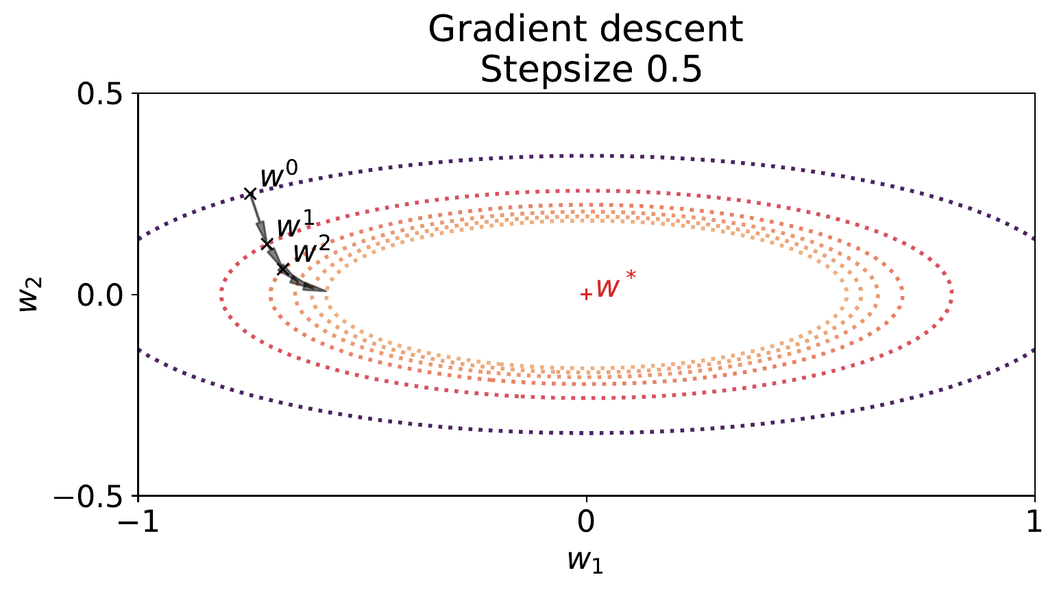
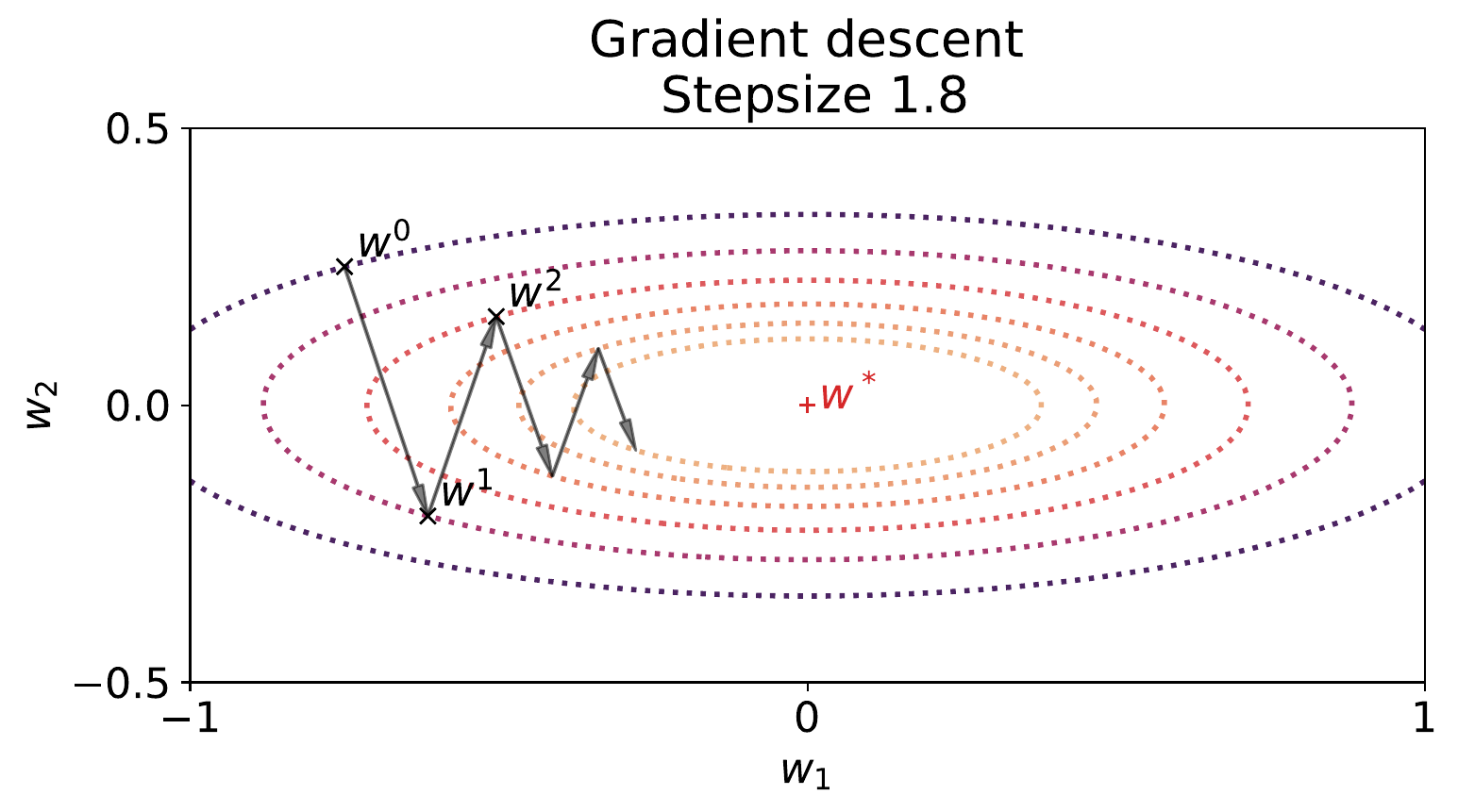
Figure 16.1: Trajectory taken by gradient descent on the objective $f (w) ≔ 0.05 w_{1}^{2} + 0.5 w_{2}^{2}$ f(w):=0.05w12+0.5w22 with a small (left) or large (right) stepsize. In each case, the iterates follow the normal vectors to the contour lines (dashed lines): the negative gradients. A small stepsize leads to slow convergence but a larger stepsize induces oscillations.

16.1.1 Variational perspective

Consider the linear approximation of $L (w)$ L(w) around $w^{t}$ wt, $L (w) \approx L (w^{t}) + ⟨ \nabla L (w^{t}), w - w^{t} ⟩ .$ L(w)≈L(wt)+⟨∇L(wt),w−wt⟩. One can easily check that the gradient descent update in Eq. (16.1) can be rewritten as the solution of a minimization problem, namely, $\begin{matrix} w^{t + 1} = \underset{w \in W}{arg min} L (w^{t}) + ⟨ \nabla L (w^{t}), w - w^{t} ⟩ + \frac{1}{2 γ} ∥ w - w^{t} ∥_{2}^{2} . & (16.2) \end{matrix}$ wt+1=w∈WargminL(wt)+⟨∇L(wt),w−wt⟩+2γ1∥w−wt∥22.(16.2) In words, a gradient descent update optimizes a trade-off between staying close to the current $w^{t}$ wt, thanks to the proximity term $\frac{1}{2 γ} ∥ w - w^{t} ∥_{2}^{2}$ 2γ1∥w−wt∥22, and minimizing the linearization of $L$ L around $w^{t}$ wt. Intuitively, by choosing $γ$ γ sufficiently small, we ensure that the minimizer of the regularized linear approximation stays in a neighborhood where the linear approximation is valid. This viewpoint is useful to motivate gradient descent extensions.

16.1.2 Convergence for smooth functions

As long as $\nabla L (w^{t}) \neq 0$ ∇L(wt)=0, the function $L_{t} (γ) ≔ L (w^{t} - γ \nabla L (w^{t}))$ Lt(γ):=L(wt−γ∇L(wt)) has a negative derivative at 0, i.e., $L_{t}^{'} (0) = - ∥ \nabla L (w^{t}) ∥_{2}^{2}$ Lt′(0)=−∥∇L(wt)∥22. Hence, as long as $\nabla L (w^{t}) \neq 0$ ∇L(wt)=0, there exists a stepsize ensuring a decrease in objective values at each iterate. However, without further assumptions, such a stepsize may depend on each iterate and may be infinitesimally small. To quantify the convergence of gradient descent with a constant stepsize, we restrict to the class of smooth functions. By applying Proposition 15.1 on the iterate of gradient descent, we obtain that $L (w^{t + 1}) \leq L (w^{t}) - γ ∥ \nabla L (w^{t}) ∥_{2}^{2} + \frac{β γ^{2}}{2} ∥ \nabla L (w^{t}) ∥_{2}^{2} .$ L(wt+1)≤L(wt)−γ∥∇L(wt)∥22+2βγ2∥∇L(wt)∥22. Therefore, for $β$ β-smooth functions, by selecting $γ \leq \frac{1}{β}$ γ≤β1, we get that $L (w^{t + 1}) - L (w^{t}) \leq - \frac{γ}{2} ∥ \nabla L (w^{t}) ∥_{2}^{2},$ L(wt+1)−L(wt)≤−2γ∥∇L(wt)∥22, which illustrates the main mechanism behind gradient descent: each iteration decreases the objective by a constant times the norm of the gradient of the current iterate. This equation can further be summed over all iterates up to $T$ T. This telescopes the objective values, leading to $\begin{matrix} \min_{t \in {0, \dots, T - 1}} ∥ \nabla L (w^{t}) ∥_{2}^{2} & \leq \frac{1}{T} \sum_{t = 0}^{T - 1} ∥ \nabla L (w^{t}) ∥_{2}^{2} \\ \leq \frac{2}{γ T} (L (w^{0}) - L (w^{T})) \\ \leq \frac{2}{γ T} (L (w^{0}) - L^{⋆}), \end{matrix}$ t∈{0,…,T−1}min∥∇L(wt)∥22≤T1t=0∑T−1∥∇L(wt)∥22≤γT2(L(w0)−L(wT))≤γT2(L(w0)−L⋆), where we recall that $L^{⋆}$ L⋆ is the infimum of $L$ L. Therefore, after sufficiently many iterations, gradient descent finds a point whose gradient norm is arbitrarily small.

Non-convex case

Without further assumptions, i.e., in the non-convex case, the above result (i.e., convergence to a stationary point, measured by the gradient norm) is the best we may get in theory. Denoting $T_{s} (ε)$ Ts(ε) the number of iterations needed for a gradient descent to output a point that is $ε$ ε-stationary, i.e., $∥ \nabla L (\hat{w}) ∥_{2} \leq ε$ ∥∇L(w^)∥2≤ε, we have $T_{s} (ε) \leq O (ε^{- 2})$ Ts(ε)≤O(ε−2).

Convex case

By adding a convexity assumption on the objective, we can use the lower bound provided by the convexity assumption to ensure convergence to a minimum. Namely, for a $β$ β-smooth and convex function $f$ f, and with stepsize $γ \leq 1 / β$ γ≤1/β, we have that (Nesterov, 2018) $L (w^{T}) - L^{⋆} \leq \frac{1}{γ T} ∥ w^{0} - w^{⋆} ∥_{2}^{2} .$ L(wT)−L⋆≤γT1∥w0−w⋆∥22. That is, we get a sublinear convergence rate, and the associated computational complexity to find a minimum is $T (ε) = O (1 / ε)$ T(ε)=O(1/ε).

Strongly convex case

If we further strengthen the assumptions by considering $β$ β-smooth, $μ$ μ-strongly convex functions, the convergence rate of a gradient descent can be shown to be (Nesterov, 2018), for any stepsize $γ \leq 1 / β$ γ≤1/β, $\begin{matrix} L (w^{T}) - L^{⋆} & \leq {(1 - γ μ)}^{T} (L (w^{0}) - L^{⋆}) \\ \leq \exp (- γ μ T) (L (w^{0}) - L^{⋆}) . \end{matrix}$ L(wT)−L⋆≤(1−γμ)T(L(w0)−L⋆)≤exp(−γμT)(L(w0)−L⋆). That is, we obtain a linear convergence rate and the associated computational complexity is $T (ε) = O (\ln ε^{- 1})$ T(ε)=O(lnε−1). The above convergence rates may be further refined (Nesterov, 2018); we focused above on the simplest result for clarity.

Strong convexity can also be replaced by a weaker assumption, gradient-dominating property (Polyak, 1963), i.e., $∥ \nabla L (v) ∥_{2}^{2} \geq c (L (v) - L^{⋆})$ ∥∇L(v)∥22≥c(L(v)−L⋆) for some constant $c$ c and any $v \in W$ v∈W. A convex, gradient-dominating function can also be minimized at a linear rate.

16.1.3 Momentum and accelerated variants

We started with gradient descent as a simple example of first-order optimization algorithm. However, different optimization algorithms can be designed from the access to first-order oracles and the knowledge of the class of functions considered. For example, consider quadratic convex functions $w \mapsto \frac{1}{2} w^{⊤} A w + b^{⊤} w$ w↦21w⊤Aw+b⊤w, that are a basic example of smooth strongly convex functions if $A$ A is positive definite. An optimal method in this case is the heavy-ball method of Polyak (1964), that can be written as $\begin{matrix} v^{t + 1} & ≔ ν v^{t} - γ \nabla L (w^{t}) \\ w^{t + 1} & ≔ w^{t} + v^{t + 1} . \end{matrix}$ vt+1wt+1:=νvt−γ∇L(wt):=wt+vt+1. The heavy-ball method uses an additional variable $v^{t}$ vt, that can be interpreted as the velocity of a ball driven by the negative gradient to converge towards a minimum. Intuitively, this additional velocity circumvents the oscillations that a gradient descent may present as illustrated in Fig. 16.2 compared to Fig. 16.1. For $ν = 0$ ν=0, we recover usual gradient descent. For $ν > 0$ ν>0, the velocities accumulate a form of an inertia momentum, where $ν$ ν is interpreted as the “mass” of the ball. In terms of convergence rates, the heavy-ball method can be shown to converge linearly similarly to gradient descent, but with a rate $O (\exp (- T \sqrt{μ / β}))$ O(exp(−Tμ/β)) for appropriate choices of $ν, γ$ ν,γ. In comparison, by choosing an optimal stepsize for the gradient descent, its convergence rate is $O (\exp (- T μ / β))$ O(exp(−Tμ/β)) which is provably worse, as we always have $μ / β \leq 1$ μ/β≤1.

Beyond the case of quadratic functions, accelerated variants of gradient descent for convex or strongly convex functions have been developed by Nesterov (2018). Such variants have inspired the design of optimization algorithms in stochastic settings presented below.

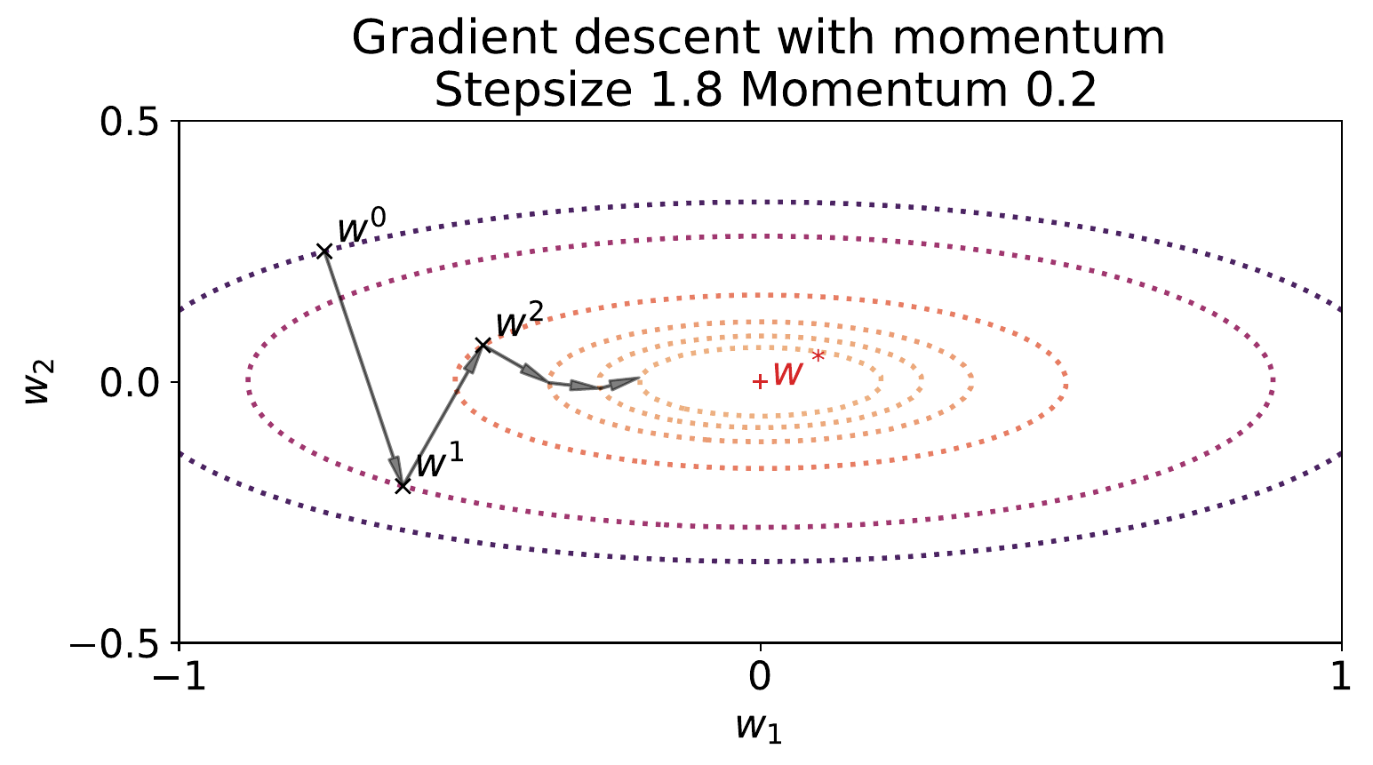
Figure 16.2: Trajectory taken by gradient descent with momentum. Compared to gradient descent without momentum, for the same stepsize, the oscillations previously observed in Fig. 16.1 are no longer present, and the algorithm converges faster to the minimum.

16.2 Stochastic gradient descent

In machine learning, we are usually interested in minimizing the expected loss of the model over the data distribution $ρ$ ρ: $\min_{w \in W} L (w) ≔ E_{S \sim ρ} [L (w; S)] .$ w∈Wmin L(w):=ES∼ρ[L(w;S)]. For example, $L$ L is often set to $L (w; S) ≔ ℓ (Y, f (X, w))$ L(w;S):=ℓ(Y,f(X,w)), where $ℓ$ ℓ is a loss function, $f$ f is a neural network and $S = (X, Y)$ S=(X,Y) is a random pair, composed of an input $X$ X and an associated target $Y$ Y, sampled from $ρ$ ρ. In this setting, since the data distribution $ρ$ ρ is generally unknown and may be infinite, we cannot exactly evaluate the expected loss $L (w)$ L(w) or its gradient $\nabla L (w)$ ∇L(w).

In practice, we are often given a fixed dataset of $n$ n pairs $s_{i} = (x_{i}, y_{i})$ si=(xi,yi). This is a special case of the expected loss setting, since this can be seen as an empirical distribution $ρ = ρ_{n}$ ρ=ρn $L (w) = E_{S \sim ρ_{n}} [L (w; S)] = \frac{1}{n} \sum_{i = 1}^{n} L (w; (X_{i}, Y_{i})) .$ L(w)=ES∼ρn[L(w;S)]=n1i=1∑nL(w;(Xi,Yi)). The gradient of $L (w)$ L(w) is then $\nabla L (w) ≔ \frac{1}{n} \sum_{i = 1}^{n} \nabla L (w; (x_{i}, y_{i})) .$ ∇L(w):=n1i=1∑n∇L(w;(xi,yi)). In this case, we see that the full gradient $\nabla L (w)$ ∇L(w), as needed by gradient descent, is the average of the individual gradients. That is, the cost of computing $\nabla L (w)$ ∇L(w) is proportional to the number of training points $n$ n. For $n$ n very large, that is a very large amount of samples, this computational cost can be prohibitive. Stochastic gradients circumvent this issue.

16.2.1 Stochastic gradients

Usually, even if we do not know $ρ$ ρ, we can sample from it, i.e., we have access to samples $S \sim ρ$ S∼ρ. We can then use a stochastic gradient of the form $\nabla L (w; S)$ ∇L(w;S) as a random estimate of $\nabla L (w)$ ∇L(w). This may look like a rough estimate but, on average, this is a valid approximation since $E_{S \sim ρ} [\nabla L (w; S)] = \nabla L (w) .$ ES∼ρ[∇L(w;S)]=∇L(w). We say that $\nabla L (w; S)$ ∇L(w;S) is an unbiased estimator of $\nabla L (w)$ ∇L(w). To further improve the approximation, we may also consider mini-batch estimates by sampling $m ≪ n$ m≪n data points $S_{i} ≔ (X_{i}, Y_{i})$ Si:=(Xi,Yi) and using $\frac{1}{m} \sum_{i = 1}^{m} \nabla L (w; S_{i})$ m1∑i=1m∇L(w;Si), whose expectation still matches $\nabla L (w)$ ∇L(w), while potentially reducing the approximation error by averaging multiple stochastic gradients. Computationally, the main advantage is that the cost is now proportional to $m$ m instead of $n$ n.

In whole generality, one can consider stochastic first-order oracles defined below.

Definition 16.1 (Stochastic first-order oracles)

A stochastic first-order oracle of an expected objective $L (w)$ L(w) is a random estimate $g (w; S)$ g(w;S) of $\nabla L (w)$ ∇L(w) with $S$ S sampled according to some distribution $q$ q. A stochastic gradient is said to be an unbiased estimator if $E_{S \sim q} [g (w; S)] = \nabla L (w) .$ ES∼q[g(w;S)]=∇L(w). The variance of a stochastic gradient is $E_{S \sim q} [{∥ g (w; S) - \nabla L (w) ∥}_{2}^{2}] .$ ES∼q[∥g(w;S)−∇L(w)∥22].

When $q = ρ$ q=ρ, we recover stochastic gradients. When $q$ q is the product of $m$ m independent samples according to $p$ p, we recover mini-batch stochastic gradients. First-order stochastic optimization algorithms build upon stochastic first-order oracles to approximately find the minimum of the expected objective. In such a setting, the iterates of the algorithm are by definition random. Convergence rates therefore need to be expressed in probabilistic terms by considering for example the expected objective value according to the randomness of the oracles.

16.2.2 Vanilla SGD

Equipped with a stochastic first-order oracle, such as (mini-batch) stochastic gradients, we can define stochastic gradient descent as $w^{t + 1} = w^{t} - γ g (w^{t}; S^{t}) where S^{t} \sim q .$ wt+1=wt−γg(wt;St)where St∼q. We assume that $S^{t}$ St is independent of $w^{t}$ wt. Compared to the usual gradient descent, the main impediment of the stochastic setting is the additional noise induced by the stochastic estimates: their variance.

For example, consider applying a stochastic gradient descent on the expectation of $β$ β-smooth convex functions $L (w; s)$ L(w;s) with unbiased oracles. To harness the randomness of the iterates, consider after $T$ T iterations outputting the average of the first $T$ T iterates, that is ${\overset{ˉ}{w}}^{T} ≔ \frac{1}{T} \sum_{t = 1}^{T} w^{t}$ wˉT:=T1∑t=1Twt. Moreover, suppose that the variance of the stochastic first-order oracles is bounded by $σ^{2}$ σ2 for all minimizers $w^{⋆}$ w⋆ of $L$ L. Denoting by $E_{S_{0}, \dots, S_{T - 1}}$ ES0,…,ST−1 the randomness associated to the stochastic oracles, we have then that for a stepsize $γ \leq 1 / (4 β)$ γ≤1/(4β) (Lan, 2012), $E_{S_{0}, \dots, S_{T - 1}} [L ({\overset{ˉ}{w}}^{T})] - L^{⋆} \leq \frac{1}{γ T} ∥ w_{0} - w^{⋆} ∥_{2}^{2} + 2 γ σ^{2} .$ ES0,…,ST−1[L(wˉT)]−L⋆≤γT1∥w0−w⋆∥22+2γσ2. The resulting convergence rate illustrates that a stochastic gradient descent converges to the minimum of the expected objective up to a constant term depending on the variance of the oracle and the stepsize. One can diminish the variance by considering mini-batches: if the variance of a single stochastic gradient is $σ_{1}^{2}$ σ12, considering a mini-batch of $m$ m gradients reduces the variance of the corresponding oracle to $σ_{m}^{2} = σ_{1}^{2} / m$ σm2=σ12/m. To decrease the additional term, one may also decrease the stepsizes over the iterations. For example, by choosing a decreasing stepsize like $γ^{t} = t^{- 1 / 2}$ γt=t−1/2, the convergence rate is then of the order $O ((∥ w_{0} - w^{⋆} ∥_{2}^{2} + σ^{2} \ln t) / \sqrt{t})$ O((∥w0−w⋆∥22+σ2lnt)/t). The stepsize can also be selected as a constant $γ_{0}$ γ0 that decreases the average objective for the first $T_{0}$ T0 iterations and is reduced by a multiplicative factor at regular intervals like $γ_{j} = ρ γ_{j - 1}$ γj=ργj−1 for $ρ \in (0, 1)$ ρ∈(0,1) to handle iterations between $T_{j}, T_{j + 1}$ Tj,Tj+1. Alternative stepsize schedules such as a cosine decay (Loshchilov and Hutter, 2016) have recently become popular.

The literature on alternative optimization schemes for stochastic optimization is still rapidly evolving, with new heuristics regularly proposed. We present below two popular techniques.

16.2.3 Momentum variants

Accelerated optimization algorithms developed in the deterministic setting may be extended to the stochastic setting. For example, the heavy-ball method can be adapted to the stochastic setting, leading to stochastic gradient descent with momentum (Sutskever et al., 2013) generally implemented as $\begin{matrix} v^{t + 1} & ≔ ν v^{t} + g (w^{t}; S^{t}) \\ w^{t + 1} & ≔ w^{t} - γ v^{t + 1} . \end{matrix}$ vt+1wt+1:=νvt+g(wt;St):=wt−γvt+1. As mentioned earlier the momentum method can be modified to handle non-quadratic smooth strongly convex functions. This leads to Nesterov’s accelerated method in the deterministic setting. This has been adapted to the stochastic setting with a so-called Nesterov momentum (Sutskever et al., 2013) $\begin{matrix} v^{t + 1} & ≔ ν v^{t} + g (w^{t} - γ ν v^{t}; S^{t}) \\ w^{t + 1} & ≔ w^{t} - γ v^{t + 1} . \end{matrix}$ vt+1wt+1:=νvt+g(wt−γνvt;St):=wt−γvt+1.

16.2.4 Adaptive variants

In any gradient descent-like algorithm, selecting the stepsize is key for good performance. While a constant stepsize may be used if the function is smooth, we may not know in advance the smoothness constant of the objective, which means that additional procedures may be required to select appropriately the stepsize. In the deterministic case, line-searches such as the Armijo or Wolfe’s rules (Wright and Nocedal, 1999) can be used to check whether the selected stepsize sufficiently decreases the objective at each iteration. Such rules have been adapted in the stochastic setting (Vaswani et al., 2019).

Another way to decrease the sensitivity of the algorithm with respect to the stepsize has been to estimate first- and second-order moments of the gradients and use the latter as a form of preconditioning to smooth the trajectory of the iterates. This led to the popular Adam optimizer (Kingma and Ba, 2014). It takes the form, $\begin{matrix} m^{t + 1} & ≔ ν_{1} m^{t} + (1 - ν_{1}) g^{t} \\ v^{t + 1} & ≔ ν_{2} v^{t} + (1 - ν_{2}) (g^{t})^{2} \\ {\hat{m}}^{t} & ≔ m^{t} / (1 - ν_{1}^{t}) \\ {\hat{v}}^{t} & ≔ v^{t} / (1 - ν_{2}^{t}) \\ w^{t + 1} & ≔ w^{t} - γ {\hat{m}}^{t + 1} / (\sqrt{{\hat{v}}^{t + 1}} + ε), \end{matrix}$ mt+1vt+1m^tv^twt+1:=ν1mt+(1−ν1)gt:=ν2vt+(1−ν2)(gt)2:=mt/(1−ν1t):=vt/(1−ν2t):=wt−γ m^t+1/(v^t+1+ε), where $g^{t} ≔ g (w^{t}; S^{t})$ gt:=g(wt;St), $(g^{t})^{2}$ (gt)2 denotes the element-wise square of $g^{t}$ gt and $ν_{1}, ν_{2}, γ, ε$ ν1,ν2,γ,ε are hyper-parameters of the algorithm. Numerous variants exist, such as varying the stepsize $γ$ γ above along the iterations.

16.3 Projected gradient descent

Oftentimes, we seek to find the solution of a minimization problem subject to constraints on the variables, of the form $\begin{matrix} \min_{w \in C} L (w), & (16.3) \end{matrix}$ w∈CminL(w),(16.3) where $C \subseteq W = R^{P}$ C⊆W=RP is a set of constraints. We say that an approximate solution $\hat{w}$ w to Eq. (16.3) is feasible if $\hat{w} \in C$ w∈C. Naturally, the design of algorithms for the constrained setting now depends, not only on information about $L$ L, but also on information about $C$ C.

Similarly to $L$ L, different oracles can be considered about $C$ C. One of the most commonly used oracles is the Euclidean projection

Definition 16.2 (Euclidean projection)

The Euclidean projection onto the set $C$ C is defined by ${p r o j}_{C} (w) ≔ \underset{v \in C}{arg min} ∥ w - v ∥_{2}^{2} .$ projC(w):=v∈Cargmin∥w−v∥22.

This projection, which is well-defined when $C$ C is a convex set, can be used in projected gradient descent, that we briefly review below. Typically, the projection on a particular set $C$ C requires a dedicated algorithm to compute it.

Other possible oracles are linear maximization oracles (LMO) used in Frank-Wolfe algorithms and Bregman projection oracles, used in mirror descent algorithms. The algorithm choice can be dictated by what oracle about $C$ C is available.

16.3.1 Variational perspective

Projected gradient descent is a natural generalization of gradient descent, based on the Euclidean projection oracle. Its iterates read $w^{t + 1} ≔ {p r o j}_{C} (w^{t} - γ \nabla L (w^{t})) .$ wt+1:=projC(wt−γ∇L(wt)). At each iteration, we attempt to decrease the objective by moving along the negative gradient direction, while ensuring that the next iterate remains feasible, thanks to the projection step.

Similarly to the variational perspective of gradient descent in Eq. (16.2), the projected gradient descent update is equivalent to $w^{t + 1} = \underset{w \in C}{arg min} L (w^{t}) + ⟨ \nabla L (w^{t}), w - w^{t} ⟩ + \frac{1}{2 γ} ∥ w - w^{t} ∥_{2}^{2} .$ wt+1=w∈CargminL(wt)+⟨∇L(wt),w−wt⟩+2γ1∥w−wt∥22. This shows that projected gradient descent minimizes a trade-off between staying close to $w^{t}$ wt and minimizing the linearization of $L$ L around $w^{t}$ wt, while staying in $C$ C.

In terms of convergence rates, they remain the same as gradient descent (Nesterov, 2018). For example, projected gradient descent on a smooth convex function still converges at a rate $R (T) = O (1 / T)$ R(T)=O(1/T).

There are numerous extensions of vanilla projected gradient descent. Similarly to gradient descent, the stepsize can be automatically adjusted using linesearch techniques and there exists accelerated variants. If we replace $\nabla L (w)$ ∇L(w) with a stochastic gradient $\nabla L (w; S)$ ∇L(w;S), we obtain a stochastic projected gradient descent.

16.3.2 Optimality conditions

In the unconstrained case, a minimum necessarily has a zero gradient. In the constrained setting, there may not be any feasible parameters with zero gradient. Instead, the optimality of a point is characterized by the fact that no better solution can be found by moving along the gradient at that point, while staying in the constraints. Formally, it means that for any $γ > 0$ γ>0, a minimizer $w^{⋆}$ w⋆ of $L$ L on $C$ C satisfies $w^{⋆} = {p r o j}_{C} (w^{⋆} - γ \nabla L (w^{⋆})) .$ w⋆=projC(w⋆−γ∇L(w⋆)). It can be shown that this condition is equivalent (Nesterov, 2018) to $⟨ \nabla L (w^{⋆}), w - w^{⋆} ⟩ \geq 0 \forall w \in C .$ ⟨∇L(w⋆),w−w⋆⟩≥0∀w∈C.

16.3.3 Commonly used projections

We now briefly review a few useful Euclidean projections.

If $C = R^{P}$ C=RP, we obviously have ${p r o j}_{C} (w) = w .$ projC(w)=w. Therefore, in the unconstrained setting, projected gradient descent indeed recovers gradient descent.
If $C = [a, b]^{P}$ C=[a,b]P (box constraints), we have ${p r o j}_{C} (w) = c l i p (w, a, b) ≔ \min {\max {w, a}, b} .$ projC(w)=clip(w,a,b):=min{max{w,a},b}. where the $\min$ min and $\max$ max are applied coordinate-wise.
As a special case of the above, if $C = R_{+}^{P}$ C=R+P (non-negative orthant), ${p r o j}_{C} (w) = \max {w, 0},$ projC(w)=max{w,0}, also known as non-negative part or ReLU.
If $C = △^{P}$ C=△P (unit probability simplex), ${p r o j}_{C} (w) = \max {w - τ 1, 0},$ projC(w)=max{w−τ1,0}, where $τ \in R$ τ∈R is a constant ensuring that ${p r o j}_{C} (w)$ projC(w) normalizes to $1$ 1. It is known that $τ$ τ can be found in $O (P \log P)$ O(PlogP) using a sort. This can be improved to $O (P)$ O(P) using a median-finding like algorithm.

16.4 Proximal gradient method

The constrained setting (with $C$ C a convex set) can be recast as unconstrained optimization, by extending our analysis to functions taking infinite values. Let us denote the indicator function of the set $C$ C by $ι_{C} (w) ≔ {\begin{matrix} 0 & if w \in C \\ + \infty & otherwise \end{matrix} .$ ιC(w):={0+∞if w∈Cotherwise. Clearly, the constrained problem in Eq. (16.3) can then be rewritten as $\min_{w \in W} L (w) + ι_{C} (w) .$ w∈WminL(w)+ιC(w). This suggests that constrained optimization is a special case of composite objectives of the form $\min_{w \in W} L (w) + Ω (w),$ w∈WminL(w)+Ω(w), where $Ω$ Ω is a convex but potentially non-differentiable function. We assume that we have access to an oracle associated with $Ω$ Ω called the proximal operator.

Definition 16.3 (Proximal operator)

The proximal operator associated with $Ω ⁣ : W \to R$ Ω:W→R is ${p r o x}_{Ω} (w) ≔ \underset{v \in W}{arg min} \frac{1}{2} ∥ w - v ∥_{2}^{2} + Ω (v) .$ proxΩ(w):=v∈Wargmin21∥w−v∥22+Ω(v).

This leads to the proximal gradient method, reviewed below.

16.4.1 Variational perspective

With this method, the update reads $w^{t + 1} = {p r o x}_{γ Ω} (w^{t} - γ \nabla L (w^{t})) .$ wt+1=proxγΩ(wt−γ∇L(wt)). This update again enjoys an intuitive variational perspective, namely, $w^{t + 1} = \underset{w \in W}{arg min} L (w^{t}) + ⟨ \nabla L (w^{t}), w - w^{t} ⟩ + \frac{1}{2 γ} ∥ w - w^{t} ∥_{2}^{2} + Ω (w) .$ wt+1=w∈WargminL(wt)+⟨∇L(wt),w−wt⟩+2γ1∥w−wt∥22+Ω(w). That is, we linearize $L$ L around $w^{t}$ wt, but keep $Ω$ Ω as is.

The proximal gradient method is popularly used when the objective function contains a sparsity-inducing regularizer $Ω$ Ω. For example, for the LASSO (Tibshirani, 1996), which aims at predicting targets $y = (y_{1}, \dots, y_{n})^{⊤} \in R^{N}$ y=(y1,…,yn)⊤∈RN from observations $X = (x_{1}, \dots, x_{n})^{⊤} \in R^{N \times P}$ X=(x1,…,xn)⊤∈RN×P, we set $L (w) = \frac{1}{2} ∥ X w - y ∥_{2}^{2}$ L(w)=21∥Xw−y∥22 and $Ω (w) = λ ∥ w ∥_{1}$ Ω(w)=λ∥w∥1, where $λ > 0$ λ>0 controls the regularization strength. In this case, ${p r o x}_{Ω}$ proxΩ is the so-called soft-thresholding operator (see below).

Convergence guarantees of the proximal gradient method remain the same as for gradient descent, such as a $O (1 / T)$ O(1/T) rate for smooth convex functions.

16.4.2 Optimality conditions

An optimal solution of the problem is characterized by the fixed point equation $w^{⋆} = {p r o x}_{γ Ω} (w^{⋆} - γ \nabla L (w^{⋆})),$ w⋆=proxγΩ(w⋆−γ∇L(w⋆)), for all $γ > 0$ γ>0 (Nesterov, 2018). In other words, the proximal gradient method (which includes gradient descent and projected gradient descent as special cases), can be seen as fixed point iteration schemes. Such a viewpoint suggests using acceleration methods from the fixed point literature such as Anderson acceleration (Pollock and Rebholz, 2021). It is also useful when designing implicit differentiation schemes as presented in Chapter 8.

16.4.3 Commonly-used proximal operators

We now briefly review a few useful proximal operators.

If $Ω (w) = 0$ Ω(w)=0, we have ${p r o x}_{γ Ω} (w) = w .$ proxγΩ(w)=w. Therefore, with this proximal operator, the proximal gradient method recovers gradient descent.
If $Ω (w) = ι_{C} (w)$ Ω(w)=ιC(w), we have ${p r o x}_{γ Ω} (w) = {p r o j}_{C} (w) .$ proxγΩ(w)=projC(w). Therefore, with this proximal operator, the proximal gradient method recovers projected gradient descent.
If $Ω (w) = λ ∥ w ∥_{1}$ Ω(w)=λ∥w∥1, we have ${p r o x}_{γ Ω} (w) = (s i g n (w) \cdot \max (∣ w ∣ - γ λ, 0)),$ proxγΩ(w)=(sign(w)⋅max(∣w∣−γλ,0)), where the operations are applied coordinate-wise. This is the so-called soft-thresholding operator.
$Ω (w) = λ \sum_{g \in G} ∥ w_{g} ∥_{2}$ Ω(w)=λ∑g∈G∥wg∥2 where $G$ G is a partition of $[P]$ [P] and $w_{g}$ wg denotes the subvector restricted to $g$ g, then we have ${[{p r o x}_{γ Ω} (w)]}_{g} = \max (1 - λ \cdot γ / ∥ w_{g} ∥_{2}, 0) w_{g},$ [proxγΩ(w)]g=max(1−λ⋅γ/∥wg∥2,0)wg, which is used in the group lasso (Yuan and Lin, 2006) and can be used to encourage group sparsity.

For a review of more proximal operators, see for instance (Bach et al., 2012; Parikh et al., 2014).

16.5 Summary

From a variational perspective, gradient descent is the algorithm obtained when linearizing the objective function and using a quadratic regularization term.
Projected gradient descent is the algorithm obtained when there is an additional constraint (the Euclidean projection naturally appearing, due to the quadratic regularization term).
When the objective is the sum of a differentiable function and a non-differentiable function, proximal gradient is the algorithm obtained when the differentiable function is linearized but the non-differentiable function is kept as is.
We also reviewed various stochastic gradient based algorithms, including vanilla SGD, SGD with momentum and Adam.

GeezerVison