Chapter 17Second-order optimization

We review in this chapter methods whose iterations take the form $w^{t + 1} ≔ w^{t} - γ^{t} B^{t} \nabla L (w^{t}),$ wt+1:=wt−γtBt∇L(wt), where $γ^{t}$ γt is a stepsize and $B^{t}$ Bt is a pre-conditioning matrix involving second-order derivatives.

17.1 Newton’s method

17.1.1 Variational perspective

We saw in Eq. (16.2) that gradient descent can be motivated from a variational perspective, in which we use a linear approximation of the objective around the current iterate, obtained from the current gradient. Similarly, if we have access not only to the gradient but also to the Hessian of the objective, we can use a quadratic approximation of the objective around the current iterate. More precisely, given a function $L (w)$ L(w), we may consider minimizing the second-order Taylor approximation of $L (w)$ L(w) around the current iterate $w^{t}$ wt, $L (w) \approx L (w^{t}) + ⟨ \nabla L (w^{t}), w - w^{t} ⟩ + \frac{1}{2} ⟨ w - w^{t}, \nabla^{2} L (w^{t}) (w - w^{t}) ⟩ .$ L(w)≈L(wt)+⟨∇L(wt),w−wt⟩+21⟨w−wt,∇2L(wt)(w−wt)⟩. Newton’s method simply iteratively minimizes this quadratic approximation around the current iteration $w^{t}$ wt, namely, $\begin{matrix} w^{t + 1} = \underset{w \in W}{arg min} L (w^{t}) + ⟨ \nabla L (w^{t}), w - w^{t} ⟩ + \frac{1}{2} ⟨ w - w^{t}, \nabla^{2} L (w^{t}) (w - w^{t}) ⟩ . \end{matrix}$ wt+1=w∈WargminL(wt)+⟨∇L(wt),w−wt⟩+21⟨w−wt,∇2L(wt)(w−wt)⟩.(17.1) If the Hessian is positive definite at $w^{t}$ wt, which we denote by $\nabla^{2} L (w^{t}) ≻ 0$ ∇2L(wt)≻0, then the minimum is well-defined and unique (this is for example the case if $L$ L is strictly convex). The iterates can then be written analytically as $w^{t + 1} = w^{t} - \nabla^{2} L (w^{t})^{- 1} \nabla L (w^{t}) .$ wt+1=wt−∇2L(wt)−1∇L(wt). If the Hessian is not positive definite, the minimum may not be defined. Ignoring this issue and taking the analytical formulation could be dangerous, as it could amount to computing the maximum of the quadratic instead if, for example, the quadratic was strictly concave (i.e., $\nabla^{2} L (w) ≺ 0$ ∇2L(w)≺0).

17.1.2 Regularized Newton method

A simple technique to circumvent this issue consists in adding a regularization term to the Hessian. Namely, from a variational viewpoint, we can add a proximity term $\frac{1}{2} ∥ w - w^{t} ∥_{2}^{2}$ 21∥w−wt∥22, encouraging it to stay close to the current $w^{t}$ wt. The iterates of this regularized Newton method then take the form $\begin{matrix} w^{t + 1} = \underset{w \in W}{arg min} & L (w^{t}) + ⟨ \nabla L (w^{t}), w - w^{t} ⟩ + \frac{1}{2} ⟨ w - w^{t}, \nabla^{2} L (w^{t}) (w - w^{t}) ⟩ \\ + \frac{η^{t}}{2} ∥ w - w^{t} ∥_{2}^{2}, \end{matrix}$ wt+1=w∈Wargmin L(wt)+⟨∇L(wt),w−wt⟩+21⟨w−wt,∇2L(wt)(w−wt)⟩+2ηt∥w−wt∥22, where $η^{t}$ ηt controls the regularization strength. Assuming $η^{t} > 0$ ηt>0 is strong enough to make $\nabla^{2} L (w^{t}) + η^{t} I$ ∇2L(wt)+ηtI positive-definite, we have $w^{t + 1} = w^{t} - d^{t},$ wt+1=wt−dt, where we defined the direction $\begin{matrix} d^{t} ≔ (\nabla^{2} L (w^{t}) + η^{t} I)^{- 1} \nabla L (w^{t}) . & (17.2) \end{matrix}$ dt:=(∇2L(wt)+ηtI)−1∇L(wt).(17.2) Other techniques to circumvent this issue include using cubic regularization and modifying the spectral decomposition of the Hessian, by thresholding the eigenvalues or taking their absolute values. We refer the interested reader to, e.g., (Nesterov, 2018; Wright and Nocedal, 1999) for more details.

17.1.3 Approximate direction

We observe a main impediment for implementing such a second-order optimization algorithm: even if we had access to the Hessian of the objective for free and this Hessian was positive definite, computing the exact direction $d^{t}$ dt in Eq. (17.2) requires computing an inverse-Hessian vector product (IHVP) with the gradient $\nabla L (w^{t})$ ∇L(wt). Doing so exactly requires solving a linear system $(\nabla^{2} L (w^{t}) + η^{t} I) d^{t} = \nabla L (w^{t}),$ (∇2L(wt)+ηtI)dt=∇L(wt), which a priori takes $O (P^{3})$ O(P3) time. In practice, however, we can compute IHVPs approximately, as explained in Section 9.4.

17.1.4 Convergence guarantees

While implementing Newton’s method comes at a higher computational cost, it can also benefit from faster convergence rates. Briefly, if Newton’s method is initialized at a point $w^{0} \in W$ w0∈W close enough to the minimizer $w^{⋆}$ w⋆ of a $μ$ μ-strongly convex function with $M$ M-Lipschitz continuous Hessian (namely $∥ w^{0} - w^{*} ∥_{2} \leq \frac{2 μ}{3 M}$ ∥w0−w∗∥2≤3M2μ), then Newton’s method converges at a quadratic rate (Nesterov, 2018), that is, $R (t) \leq O (\exp (- 2^{t}))$ R(t)≤O(exp(−2t)) (see Section 15.5 for a brief introduction to performance guarantees). This is far superior to gradient descent. Such an efficiency motivated the development of interior point methods, that have been a breakthrough in constrained optimization, thanks to the use of log-barrier penalties (Nesterov, 2018).

17.1.5 Linesearch

In practice, we may not have access to an initial point close enough to the minimizer. In that case, even for strictly convex functions for which Newton’s steps are well-defined, taking $w^{t + 1} = w^{t} - d^{t}$ wt+1=wt−dt may not ensure a decrease of the objective values. Nevertheless, the direction $d^{t}$ dt may define a descent direction as defined below.

Definition 17.1 (Descent direction)

A point $d \in W$ d∈W defines a descent direction $- d$ −d for an objective $L$ L at $w$ w, if there exists a positive stepsize $γ > 0$ γ>0 such that $L (w - γ d) \leq L (w) .$ L(w−γd)≤L(w). If $L$ L is differentiable, $- d$ −d is a descent direction if $⟨ - d, \nabla L (w) ⟩ < 0$ ⟨−d,∇L(w)⟩<0.

For Newton’s method without regularization, $d^{t} = \nabla^{2} L (w^{t})^{- 1} \nabla L (w^{t})$ dt=∇2L(wt)−1∇L(wt) is then a descent direction at $w^{t}$ wt, as long as $\nabla L (w^{t}) \neq 0$ ∇L(wt)=0 and $\nabla^{2} L (w^{t}) ≻ 0$ ∇2L(wt)≻0. If $\nabla^{2} L (w^{t}) ⊁ 0$ ∇2L(wt)≻0, choosing $η^{t} > 0$ ηt>0 such that $\nabla^{2} L (w^{t}) + η^{t} I ≻ 0$ ∇2L(wt)+ηtI≻0, also ensures that $d^{t} = - (\nabla^{2} L (w^{t}) + η^{t} I)^{- 1} \nabla L (w^{t})$ dt=−(∇2L(wt)+ηtI)−1∇L(wt) is a descent direction (as long as $\nabla L (w^{t}) \neq 0$ ∇L(wt)=0). Newton’s method is then generally equipped with a linesearch method that attempts to take steps of the form $w^{t + 1} = w^{t} - γ^{t} d^{t}$ wt+1=wt−γtdt with $γ^{t}$ γt chosen as the largest stepsize among ${ρ^{τ}, τ \in N}$ {ρτ,τ∈N} for $ρ \in (0, 1)$ ρ∈(0,1) until a sufficient decrease of the objective is satisfied such as, for $c \in (0, 1)$ c∈(0,1), $L (w^{t} - γ^{t} d^{t}) \leq L (w^{t}) - c γ^{t} ⟨ \nabla L (w^{t}), \nabla^{2} L (w^{t})^{- 1} \nabla L (w^{t}) ⟩ .$ L(wt−γtdt)≤L(wt)−cγt⟨∇L(wt),∇2L(wt)−1∇L(wt)⟩. For strongly convex functions, such an implementation exhibits two phases: a first phase during which Newton’s steps are “damped” by using a stepsize $γ^{t} < 1$ γt<1 and a second phase of super-fast convergence during which stepsizes $γ^{t} = 1$ γt=1 are taken, and the objective decreases very fast. Even far from the optimum, Newton directions can advantageously adapt to the local geometry of the objective to speed up convergence compared to a regular gradient descent as explained below.

17.1.6 Geometric interpretation

To understand the efficiency of Newton’s method compared to gradient descent, consider the minimization of a simple quadratic $L (w) = \frac{1}{2} a w_{1}^{2} + \frac{1}{2} b w_{2}^{2}$ L(w)=21aw12+21bw22 for $a ≫ b \geq 0$ a≫b≥0, as illustrated in Fig. 17.1. A gradient descent moves along the directions $\nabla L (w) = (a w_{1}, b w_{2})^{⊤}$ ∇L(w)=(aw1,bw2)⊤ and its stepsize is limited by the variations in the first coordinate leading to some oscillations. If we were simply rescaling the gradient by $(a, b)$ (a,b), i.e., taking steps of the form $w^{t + 1} = w^{t} - γ d i a g (a^{- 1}, b^{- 1}) \nabla L (w^{t}),$ wt+1=wt−γdiag(a−1,b−1)∇L(wt), the variations in both coordinates would be normalized to one and the stepsize could simply be chosen to $γ = 1$ γ=1 to directly get $w^{⋆}$ w⋆. In other words, by adapting the geometry of the directions with the geometry induced by the objective, we can circumvent the oscillations.

That’s exactly what Newton’s method does by modifying the gradient direction using the inverse of the Hessian. Formally, at iteration $t$ t, consider the modified objective $\tilde{L} (v) = L (A v) for A = \nabla^{2} L (w^{t})^{- 1 / 2},$ L~(v)=L(Av) for A=∇2L(wt)−1/2, with $L$ L strictly convex and $A$ A the inverse matrix square root of the Hessian. One easily verifies that a Newton step is equivalent to a gradient step on $\tilde{L}$ L~, that is, $v^{t + 1} = v^{t} - \nabla \tilde{L} (v^{t}) ⟺ w^{t + 1} = w^{t} - (\nabla^{2} L (w^{t}))^{- 1} \nabla L (w^{t})$ vt+1=vt−∇L~(vt) ⟺ wt+1=wt−(∇2L(wt))−1∇L(wt) where $w^{t} = A v^{t} = \nabla^{2} L (w^{t})^{- 1 / 2} v^{t} .$ wt=Avt=∇2L(wt)−1/2vt. In the geometry induced by $A$ A, the objective is generally better conditioned as illustrated in Fig. 17.1. This explains the efficiency of Newton’s method. In particular for any strongly convex quadratic, a Newton step reaches the optimum in one iteration, while a gradient step can take many more iterations.

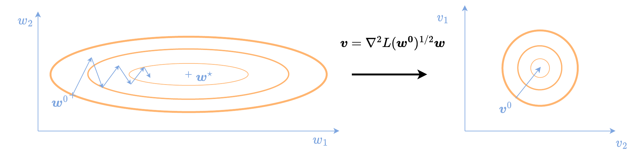
Figure 17.1: Left: Minimization of a quadratic $L (w) ≔ \frac{1}{2} a w_{1}^{2} + \frac{1}{2} b w_{2}^{2}$ L(w):=21aw12+21bw22 by gradient descent. For $a ≫ b \geq 0$ a≫b≥0, gradient descent typically oscillates. Right: minimization by Newton’s method amounts to changing the geometry of the problem to avoid oscillations.

17.1.7 Stochastic Newton’s method

Consider now an expected loss $\min_{w \in W} L (w) ≔ E_{S \sim ρ} [L (w; S)] .$ w∈Wmin L(w):=ES∼ρ[L(w;S)]. In that case, an estimate of the Hessian can be constructed just like for the gradient using that $E_{S \sim ρ} [\nabla^{2} L (w; S)] = \nabla^{2} L (w) .$ ES∼ρ[∇2L(w;S)]=∇2L(w). Les us then denote $g (w; S) \approx \nabla L (w), H (w; S^{'}) \approx \nabla^{2} L (w)$ g(w;S)≈∇L(w),H(w;S′)≈∇2L(w) some stochastic estimates of the gradient and the Hessian, respectively, with $S, S^{'}$ S,S′ independently drawn from $ρ$ ρ or from mini-batch approximations with varying mini-batch sizes. One implementation of a stochastic Newton method can then be $w^{t + 1} = w^{t} - γ^{t} (H (w^{t}; S^{'}) + η^{t} I)^{- 1} g (w^{t}; S),$ wt+1=wt−γt(H(wt;S′)+ηtI)−1g(wt;S), for $η^{t} \geq 0$ ηt≥0 such that $(H (w^{t}; S^{'}) + η^{t} I)^{- 1} ≻ 0$ (H(wt;S′)+ηtI)−1≻0 and $γ^{t}$ γt fixed or chosen to satisfy some sufficient decrease condition. We refer the interested reader to, e.g., (Xu et al., 2020), for more details and variants.

17.2 Gauss-Newton method

Newton’s method (17.1) is usually not properly defined for non-convex objective functions, since the Hessian may not be positive definite at the current iterate. We saw in Section 9.2 that the Gauss-Newton matrix can be used to define a positive-semidefinite approximation of the Hessian. Here, we revisit the Gauss-Newton method from a variational and partial linearization perspective. While the original Gauss-Newton method originates from nonlinear least-squares, we will first describe an extension to arbitrary convex loss functions, since it is both more general and easier to explain.

17.2.1 With exact outer function

Consider a composite objective of the form $L (w) ≔ ℓ (f (w)),$ L(w):=ℓ(f(w)), where $ℓ : M \to R$ ℓ:M→R is a convex function, such as a convex loss function applied on a given sample, and $f : W \to M$ f:W→M is a nonlinear function, such as a neural network with parameters $w \in W$ w∈W, evaluated on the same sample. We saw that gradient descent and Newton’s method amount to using linear and quadratic approximations of $L (w)$ L(w) around the current iterate $w^{t}$ wt, respectively. As a middle ground between the two, the Gauss-Newton method uses the linearization of $f$ f around $w^{t}$ wt $f (w) \approx f (w^{t}) + \partial f (w^{t}) (w - w^{t})$ f(w)≈f(wt)+∂f(wt)(w−wt) but keeps $ℓ$ ℓ as is to obtain the objective $\begin{matrix} w^{t + 1} & ≔ \underset{w \in W}{arg min} ℓ (f (w^{t}) + \partial f (w^{t}) (w - w^{t})) \\ = \underset{w \in W}{arg min} ℓ (\partial f (w^{t}) w + f (w^{t}) - \partial f (w^{t}) w^{t}) \\ = \underset{w \in W}{arg min} ℓ (J^{t} w + δ^{t}), \end{matrix}$ wt+1:=w∈Wargminℓ(f(wt)+∂f(wt)(w−wt))=w∈Wargminℓ(∂f(wt)w+f(wt)−∂f(wt)wt)=w∈Wargminℓ(Jtw+δt), where we defined the shorthands $J^{t} ≔ \partial f (w^{t})$ Jt:=∂f(wt) and $δ^{t} ≔ f (w^{t}) - \partial f (w^{t}) w^{t}$ δt:=f(wt)−∂f(wt)wt. We call $ℓ (J^{t} w + δ^{t})$ ℓ(Jtw+δt) the partial linearization of $L = ℓ \circ f$ L=ℓ∘f at $w^{t}$ wt, as opposed to the full linearization of $L$ L used in gradient descent.

Since the composition of a convex function and of linear function is convex, this objective is convex even if $L (w)$ L(w) is nonconvex. In practice, we often add a proximity term as regularization to define $\begin{matrix} w^{t + 1} ≔ \underset{w \in W}{arg min} ℓ (J^{t} w + δ^{t}) + \frac{η^{t}}{2} ∥ w - w^{t} ∥_{2}^{2} . & (17.3) \end{matrix}$ wt+1:=w∈Wargminℓ(Jtw+δt)+2ηt∥w−wt∥22.(17.3) We can see this update as an approximation of the proximal point update $\underset{w \in W}{arg min} L (w) + \frac{η^{t}}{2} ∥ w - w^{t} ∥_{2}^{2},$ w∈WargminL(w)+2ηt∥w−wt∥22, where $L (w)$ L(w) has been replaced by its partial linearization. Solving Eq. (17.3) using gradient-based solvers requires computing the gradient of $w \mapsto ℓ (J^{t} w + δ^{t})$ w↦ℓ(Jtw+δt), which is $w \mapsto (J^{t})^{*} \nabla ℓ (J^{t} w + δ^{t})$ w↦(Jt)∗∇ℓ(Jtw+δt). Computing this gradient by autodiff therefore requires performing a forward pass to compute the JVP $J^{t} w$ Jtw and a backward pass to compute the VJP $(J^{t})^{*} \nabla ℓ (z)$ (Jt)∗∇ℓ(z). See Section 2.3 for an introduction to these operators and Chapter 8 for an introduction to autodiff.

The Gauss-Newton method with arbitrary convex outer loss is often called modified Gauss-Newton (Nesterov, 2007) or prox-linear (Drusvyatskiy and Paquette, 2019). The classical Gauss-Newton and Levenberg-Marquardt (Levenberg, 1944; Marquardt, 1963) methods originate from nonlinear least-squares and are recovered when $ℓ (z)$ ℓ(z) is quadratic (Kelley, 1995), such as $ℓ (z) ≔ \frac{1}{2} ∥ z - y ∥_{2}^{2}$ ℓ(z):=21∥z−y∥22, for $y$ y some reference target. The Gauss-Newton method corresponds classically to not using regularization (i.e., $η^{t} = 0$ ηt=0) and the Levenberg-Marquardt method uses regularization (usually called damping, potentially changing $η^{t}$ ηt across iterations). See e.g., (Messerer et al., 2021), for a survey of different variants.

17.2.2 With approximate outer function

Another variant of the Gauss-Newton method consists in replacing the convex loss $ℓ$ ℓ with its quadratic approximation around $z^{t} ≔ f (w^{t})$ zt:=f(wt), $q^{t} (z) ≔ ℓ (z^{t}) + ⟨ \nabla ℓ (z^{t}), z - z^{t} ⟩ + \frac{1}{2} ⟨ z - z^{t}, \nabla^{2} ℓ (z^{t}) (z - z^{t}) ⟩ \approx ℓ (z)$ qt(z):=ℓ(zt)+⟨∇ℓ(zt),z−zt⟩+21⟨z−zt,∇2ℓ(zt)(z−zt)⟩≈ℓ(z) to define the update $w^{t + 1} ≔ \underset{w \in W}{arg min} q^{t} (J^{t} w + δ^{t}) + \frac{η^{t}}{2} ∥ w - w^{t} ∥_{2}^{2} .$ wt+1:=w∈Wargminqt(Jtw+δt)+2ηt∥w−wt∥22. Notice that $ℓ$ ℓ has been replaced by its quadratic approximation $q^{t}$ qt. This objective is always a convex quadratic, unlike the objective of the Newton method in Eq. (17.1), which is a priori a nonconvex quadratic, if $f$ f is nonlinear. Simple calculations show that $\begin{matrix} w^{t + 1} = \underset{w \in W}{arg min} & L (w^{t}) + ⟨ q^{t}, J^{t} (w - w^{t}) ⟩ \\ + \frac{1}{2} ⟨ w - w^{t}, (J^{t})^{*} Q^{t} J^{t} (w - w^{t}) ⟩ + \frac{η^{t}}{2} ∥ w - w^{t} ∥_{2}^{2} \end{matrix}$ wt+1=w∈Wargmin L(wt)+⟨qt,Jt(w−wt)⟩+21⟨w−wt,(Jt)∗QtJt(w−wt)⟩+2ηt∥w−wt∥22 where $q^{t} ≔ \nabla ℓ (f (w^{t})) \in M = R^{Z}, Q^{t} ≔ \nabla^{2} ℓ (f (w^{t})) \in R^{Z \times Z} .$ qt:=∇ℓ(f(wt))∈M=RZ,Qt:=∇2ℓ(f(wt))∈RZ×Z. The closed form solution is $\begin{matrix} w^{t + 1} & = w^{t} - ((J^{t})^{*} Q^{t} J^{t} + η^{t} I)^{- 1} (J^{t})^{*} q^{t} \\ = w^{t} - (\nabla_{G N}^{2} (ℓ \circ f) (w^{t}) + η^{t} I)^{- 1} \nabla L (w^{t}), \end{matrix}$ wt+1=wt−((Jt)∗QtJt+ηtI)−1(Jt)∗qt=wt−(∇GN2(ℓ∘f)(wt)+ηtI)−1∇L(wt), where we used the (generalized) Gauss-Newton matrix of $L = ℓ \circ f$ L=ℓ∘f, defined in Section 9.2.

17.2.3 Linesearch

Similarly to Newton’s method, the iterates of a Gauss-Newton method may diverge when used alone. However, the direction $- (\nabla_{G N}^{2} (ℓ \circ f) (w^{t}) + η^{t} I)^{- 1} \nabla L (w^{t})$ −(∇GN2(ℓ∘f)(wt)+ηtI)−1∇L(wt) defines a descent direction for any $η^{t} > 0$ ηt>0 and can be combined with a stepsize $γ^{t}$ γt (typically chosen using a linesearch) to obtain iterates of the form $w^{t + 1} = w^{t} - γ^{t} (\nabla_{G N}^{2} (ℓ \circ f) (w^{t}) + η^{t} I)^{- 1} \nabla L (w^{t}) .$ wt+1=wt−γt(∇GN2(ℓ∘f)(wt)+ηtI)−1∇L(wt).

17.2.4 Stochastic Gauss-Newton

In deep learning, the objective generally consists in an expectation over samples of the composition between a loss function and a network function: $L (w) = E_{S \sim ρ} [L (w; S)] = E_{(X, Y) \sim ρ} [ℓ (f (w; X); Y)]$ L(w)=ES∼ρ[L(w;S)]=E(X,Y)∼ρ[ℓ(f(w;X);Y)] where $S = (X, Y)$ S=(X,Y) denotes a sample pair of input $X$ X with associated label $Y$ Y. In that case, as already studied in Section 9.2, the Gauss-Newton matrix $\nabla_{G N}^{2} L$ ∇GN2L is the expectation of the individual Gauss-Newton matrices $\begin{matrix} \nabla_{G N}^{2} L (w; x, y) & ≔ \partial f (w; x)^{⊤} \nabla^{2} ℓ (f (w; x)) \partial f (w; x), \\ \nabla_{G N}^{2} L (w) & ≔ E_{(X, Y) \sim ρ} [\nabla_{G N}^{2} L (w; x, y)] . \end{matrix}$ ∇GN2L(w;x,y)∇GN2L(w):=∂f(w;x)⊤∇2ℓ(f(w;x))∂f(w;x),:=E(X,Y)∼ρ[∇GN2L(w;x,y)]. We can estimate the gradient and the Gauss-Newton matrix by, respectively, $g (w; S) \approx \nabla L (w)$ g(w;S)≈∇L(w), and $G (w; S^{'}) \approx \nabla_{G N}^{2} L (w)$ G(w;S′)≈∇GN2L(w) for $S, S^{'} \sim ρ$ S,S′∼ρ or using mini-batch approximations. A stochastic Gauss-Newton method therefore performs iterates $w^{t + 1} ≔ w^{t} - γ^{t} (G (w^{t}; S^{'}) + η^{t} I)^{- 1} g (w^{t}; S),$ wt+1:=wt−γt(G(wt;S′)+ηtI)−1g(wt;S), for $η^{t} \geq 0$ ηt≥0 and $γ^{t}$ γt fixed or selected to satisfy some criterion.

17.3 Natural gradient descent

Natural gradient descent (Amari, 1998) follows a similar principle as gradient descent: linearize the objective around the current iterate and minimize this approximation together with a proximity term. It differs from gradient descent in the choice of the proximity term: rather than using a squared Euclidean distance between the parameters, it uses a Kullback-Leibler divergence between the probability distributions these parameters define.

Negative log-likelihood

We consider objectives of the form $\min_{w \in W} L (w) = E_{S \sim ρ} [L (w; S)] = E_{S \sim ρ} [- \log q_{w} (S)],$ w∈WminL(w)=ES∼ρ[L(w;S)]=ES∼ρ[−logqw(S)], where $ρ$ ρ is an unknown data distribution (but from which we can sample) and where $q_{w}$ qw is a probability distribution parameterized by $w$ w. As reviewed in Chapter 3, the negative log-likelihood can be used as a loss function (many loss functions can be seen from this perspective, including the squared and logistic loss functions). In the unsupervised setting, where $S = Y$ S=Y, we simply use $q_{w} (Y)$ qw(Y) as is. In the supervised setting, where $S = (X, Y)$ S=(X,Y), we use the product rule $P (X, Y) = P (X) P (Y ∣ X)$ P(X,Y)=P(X)P(Y∣X) to parameterize $q_{w} (S)$ qw(S) as $q_{w} (x, y) ≔ ρ_{X} (x) p_{θ} (y),$ qw(x,y):=ρX(x)pθ(y), where $ρ_{X}$ ρX is the marginal distribution for $X$ X, $p_{θ} (y)$ pθ(y) is the PMF/PDF of a probability distribution and $θ = f (w; x)$ θ=f(w;x) is for instance a neural network with parameters $w \in W$ w∈W and input $x \in X$ x∈X.

17.3.1 Variational perspective

Natural gradient descent is motivated by updates of the form $w^{t + 1} = \underset{w \in W}{arg min} L (w^{t}) + ⟨ \nabla L (w^{t}), w - w^{t} ⟩ + K L (q_{w^{t}}, q_{w}),$ wt+1=w∈WargminL(wt)+⟨∇L(wt),w−wt⟩+KL(qwt,qw), where $K L (p, q) ≔ \int p (z) \log \frac{p (z)}{q (z)} d z$ KL(p,q):=∫p(z)logq(z)p(z)dz is the Kullback-Leibler (KL) divergence. Unlike gradient descent, the proximity term is therefore between the current distribution $q_{w^{t}}$ qwt and a candidate probability distribution $q_{w}$ qw. The above problem is intractable in general, as the KL may not have a closed form. Nevertheless, its quadratic approximation can be shown (Amari, 1998) to admit a simple form, $K L (q_{w^{t}}, q_{w}) \approx \frac{1}{2} ⟨ w - w^{t}, \nabla_{F}^{2} L (w^{t}) (w - w^{t}) ⟩$ KL(qwt,qw)≈21⟨w−wt,∇F2L(wt)(w−wt)⟩ where we used the Fisher information matrix $\nabla_{F}^{2} L (w)$ ∇F2L(w), studied in Section 9.3. Equipped with this quadratic approximation of the KL divergence, natural gradient descent amounts to computing iterates as $\begin{matrix} w^{t + 1} ≔ \underset{w \in W}{arg min} & L (w^{t}) + ⟨ \nabla L (w^{t}), w - w^{t} ⟩ \\ + \frac{1}{2} ⟨ w - w^{t}, \nabla_{F}^{2} L (w^{t}) (w - w^{t}) ⟩ + \frac{η^{t}}{2} ∥ w - w^{t} ∥_{2}^{2}, \end{matrix}$ wt+1:=w∈Wargmin L(wt)+⟨∇L(wt),w−wt⟩+21⟨w−wt,∇F2L(wt)(w−wt)⟩+2ηt∥w−wt∥22, where a quadratic proximity term was added to ensure a unique solution. This is a strictly convex problem as $\nabla_{F}^{2} L (w^{t})$ ∇F2L(wt) is positive semi-definite. The closed-form solution is $w^{t + 1} = w^{t} - (\nabla_{F}^{2} L (w^{t}) + η^{t} I)^{- 1} \nabla L (w^{t}) .$ wt+1=wt−(∇F2L(wt)+ηtI)−1∇L(wt). Because the Gauss-Newton and Fisher information matrices are equivalent when $p_{θ}$ pθ is an exponential family distribution (Proposition 9.6), the Gauss-Newton and natural gradient methods coincide in this case.

17.3.2 Stochastic natural gradient descent

In practice, we may not have access to $\nabla L (w^{t})$ ∇L(wt) in closed form as it is an expectation over $ρ$ ρ. Moreover, $\nabla_{F}^{2} L (w^{t})$ ∇F2L(wt) may not be computable in closed form either. To estimate the Fisher information matrix, we can use that (see Section 9.3) using the shorthand $θ ≔ f (w, X)$ θ:=f(w,X), $\nabla_{F}^{2} L (w) = E_{X \sim ρ_{X}} E_{Y \sim p_{θ}} [\nabla L (w; X, Y) \otimes \nabla L (w; X, Y)] .$ ∇F2L(w)=EX∼ρXEY∼pθ[∇L(w;X,Y)⊗∇L(w;X,Y)]. We can then build estimates $g (w^{t}; S) \approx \nabla L (w^{t}, S)$ g(wt;S)≈∇L(wt,S) and $F (w^{t}; S^{'}) \approx \nabla_{F}^{2} L (w^{t})$ F(wt;S′)≈∇F2L(wt) for $S$ S sampled from $ρ$ ρ and $S^{'}$ S′ sampled from $q_{w^{t}} (x, y) = p_{X} (x) ρ_{θ} (y)$ qwt(x,y)=pX(x)ρθ(y). A stochastic natural gradient descent can then be implemented as $w^{t + 1} = w^{t} - γ^{t} (F (w^{t}; S^{'}) + η^{t} I)^{- 1} g (w^{t}; S),$ wt+1=wt−γt(F(wt;S′)+ηtI)−1g(wt;S), where $γ^{t}$ γt is a stepsize, possibly chosen by linesearch.

In deep learning, the product with the inverse Fisher or Gauss-Newton matrices can remain costly to compute. Several approximations have been proposed, such as KFAC (Botev et al., 2017; Martens and Grosse, 2015), which uses a computationally efficient structural approximation to these matrices.

17.4 Quasi-Newton methods

17.4.1 BFGS

A celebrated example of quasi-Newton method is the BFGS method (Broyden, 1970; Fletcher, 1970; Goldfarb, 1970; Shanno, 1970), whose acronym follows from its authors’ names. The rationale of the BFGS update stems once again from a variational viewpoint. We wish to build a simple quadratic model of the objective $h^{t} (w) = L (w^{t}) + ⟨ \nabla L (w^{t}), w - w^{t} ⟩ + \frac{1}{2} ⟨ w - w^{t}, Q^{t} (w - w^{t}) ⟩$ ht(w)=L(wt)+⟨∇L(wt),w−wt⟩+21⟨w−wt,Qt(w−wt)⟩ for some $Q^{t}$ Qt built along the iterations rather than taken as $\nabla^{2} L (w^{t})$ ∇2L(wt). One desirable property of such a quadratic model would be that its gradients at consecutive iterates match the gradients of the original function, i.e., $\nabla h^{t} (w^{t}) = \nabla L (w^{t})$ ∇ht(wt)=∇L(wt) and $\nabla h^{t} (w^{t - 1}) = \nabla L (w^{t - 1})$ ∇ht(wt−1)=∇L(wt−1). A simpler condition, called the secant condition consists in considering the differences of these vectors, that is, ensuring that $\begin{matrix} \nabla h^{t} (w^{t}) - \nabla h^{t} (w^{t - 1}) = \nabla L (w^{t}) - \nabla L (w^{t - 1}) \\ ⟺ & Q^{t} (w^{t} - w^{t - 1}) = \nabla L (w^{t}) - \nabla L (w^{t - 1}) \\ ⟺ & w^{t} - w^{t - 1} = B^{t} (\nabla L (w^{t}) - \nabla L (w^{t - 1})), \end{matrix}$ ⟺⟺∇ht(wt)−∇ht(wt−1)=∇L(wt)−∇L(wt−1)Qt(wt−wt−1)=∇L(wt)−∇L(wt−1)wt−wt−1=Bt(∇L(wt)−∇L(wt−1)), for $B^{t} = (Q^{t})^{- 1}$ Bt=(Qt)−1. Building $B^{t}$ Bt, a surrogate of the inverse of the Hessian satisfying the secant equation, can then be done as $B^{t + 1} ≔ (I - ρ^{t} s^{t} (y^{t})^{⊤}) B^{t} (I - ρ^{t} s^{t} (y^{t})^{⊤}) + ρ^{t} s^{t} (s^{t})^{⊤}$ Bt+1:=(I−ρtst(yt)⊤)Bt(I−ρtst(yt)⊤)+ρtst(st)⊤ where $\begin{matrix} s^{t} & ≔ w^{t + 1} - w^{t} \\ y^{t} & ≔ \nabla L (w^{t + 1}) - \nabla L (w^{t}) \\ ρ^{t} & ≔ \frac{1}{⟨ s^{t}, y^{t} ⟩} . \end{matrix}$ stytρt:=wt+1−wt:=∇L(wt+1)−∇L(wt):=⟨st,yt⟩1. A typical implementation of BFGS stores $B^{t} \in R^{P \times P}$ Bt∈RP×P in memory, which is prohibitive when $P$ P is large.

17.4.2 Limited-memory BFGS

In practice, the limited-memory counterpart of BFGS, called LBFGS (Liu and Nocedal, 1989), is often preferred. The key observation of LBFGS is that we do not need to materialize $B^{t}$ Bt in memory: we only need to multiply it with the gradient $\nabla L (w^{t})$ ∇L(wt). That is, we can see $B^{t}$ Bt as a linear map. Fortunately, the product between $B^{t}$ Bt and any vector $v$ v can be computed efficiently if we store $(s^{1}, y^{1}, ρ^{1}), \dots, (s^{t}, y^{t}, ρ^{t})$ (s1,y1,ρ1),…,(st,yt,ρt) in memory. In practice, a small history of past values is used to reduce memory and computational cost. Because LBFGS has the benefits of second-order-like methods with much reduced cost, it has become a de-facto algorithm, outperforming most other algorithms for medium-scale problems without particular structure (Liu and Nocedal, 1989).

17.5 Approximate Hessian diagonal inverse preconditioners

One application of the approximations of the Hessian diagonal developed in Section 9.7 is to obtain cheap approximations of the Hessian diagonal inverse, $B^{t} ≔ d i a g (∣ H_{11}^{t} ∣^{- 1}, \dots, ∣ H_{P P}^{t} ∣^{- 1}) .$ Bt:=diag(∣H11t∣−1,…,∣HPPt∣−1). Such a scaling would for instance be sufficient to make the quadratic example presented in Fig. 17.1 work. Many optimization algorithms, including the popular ADAM, can be viewed as using a preconditioner that approximates the inverse of the Hessian’s diagonal.

17.6 Summary

We reviewed Newton’s method, the Gauss-Newton method, natural gradient descent, quasi-Newton methods and preconditioning methods.
We adopted a variational viewpoint, where the method’s next iterate is computed as the solution of a trade-off between minimizing an approximation of the function (linear, partially linear, quadratic) and a proximity term (squared Euclidean, KL).
All methods were shown to use iterates of the form $w^{t + 1} ≔ w^{t} - γ^{t} B^{t} \nabla L (w^{t})$ wt+1:=wt−γtBt∇L(wt) but have different trade-offs between the cost it takes to evaluate $B^{t} \nabla L (w^{t})$ Bt∇L(wt) and the richness of the information used about $L$ L.

GeezerVison