GeezerVisonThe World Wide Web, restored to 800 pixels of glory. |
| Home|About|Gaming cabinet|Archives|How it works|Starter sites |
GeezerVison is showing gr-framework.org — What can be achieved with GRPlot? — GR Framework 0.73.27 documentation What can be achieved with GRPlot?¶Plot kinds¶barplot¶A bar plot is used to display the relation between a numeric variable and a categorical variable. The resulting bars
represent the frequency or quantity of the different data categories. It can be easily created from the command line by
setting the grplot barplot.dat kind:barplot style:lined Additional key-value pairs can be included in the data header. The x- and y-columns parameter defines which columns are used for the x- and y-data. # title : Test # x_label : x # y_label : y # x_columns:1 # y_columns:2,3,4
Another example is a grplot barplot2.dat kind:barplot bar_width:1 Additional key-value pairs are included in the data header. The y-labels are applied to specific bars, while the leading number indicate how many labels there are. # title : Default style # y_labels : 7,6,10, ,3, , ,2
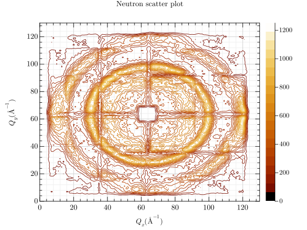
Following parameters can be used: bar_color, bar_width, bottom, columns, edge_color, edge_width, error, error_bar_style, error_columns, error_type, equal_up_and_down_error, file, grplot, ignore_blank_lines, join_plots, kind, left, orientation, right, style, title, top, twin_x, twin_y, x_flip, x_grid, x_label, x_lim, x_log, x_range, xye_file, y_columns, y_flip, y_grid, y_label, y_labels, y_lim, y_log, y_range contour¶A contour plot displays three-dimensional data over a rectangular grid. Contour lines representing different height
values are displayed depending on the specified number of # title : Neutron scatter plot # x_label : $Q_x (Å^{-1})$ # y_label : $Q_y (Å^{-1})$ To create a contour plot from the command line, set the grplot sans.dat kind:contour cmap:3
The following picture shows some other options, where the number of levels is 40 instead of 20. Any grplot sans.dat kind:contour levels:40 major_h:1003 x_log:1 cmap:3
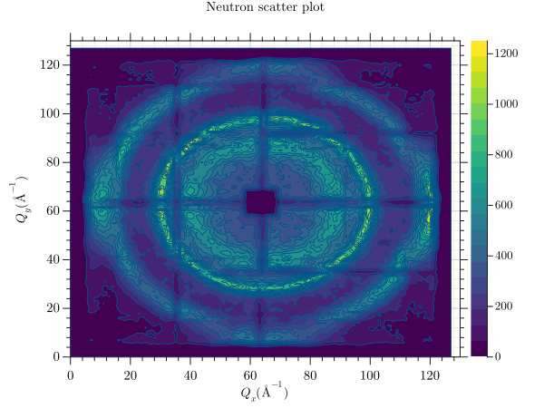
Following parameters can be used: cmap, columns, consecutive_colorbars, file, grplot, ignore_blank_lines, join_plots, keep_aspect_ratio, kind, levels, major_h, only_square_aspect_ratio, title, use_bins, x_columns, x_flip, x_grid, x_label, x_lim, x_log, x_range, xyz_file, y_columns, y_flip, y_grid, y_label, y_lim, y_log, y_range, z_lim, z_log, z_range contourf¶A contourf plot displays three-dimensional data over a rectangular mesh. Depending on the specified number of levels, contour lines representing different height values are displayed. The space between the contour lines is filled with a colour according to the specified colormap. This contour plot uses the sans dataset. The title and axis labels are defined in the data header. More information’s about the format of these files can be found under data_file. # title : Neutron scatter plot # x_label : $Q_x (Å^{-1})$ # y_label : $Q_y (Å^{-1})$ To create a filled contour plot from the command line, the grplot sans.dat kind:contourf
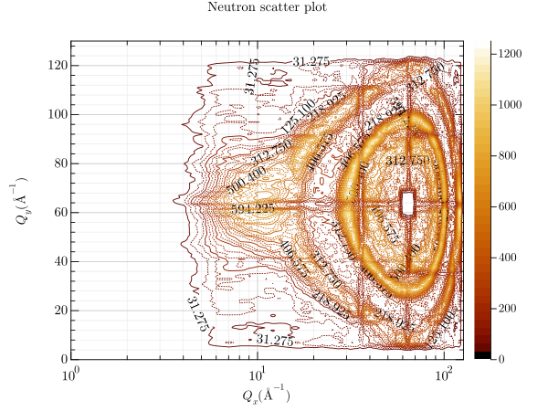
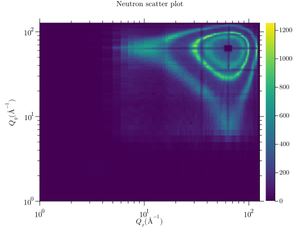
Following parameters can be used: cmap, columns, consecutive_colorbars, file, grplot, ignore_blank_lines, join_plots, keep_aspect_ratio, kind, levels, major_h, only_square_aspect_ratio, title, use_bins, x_columns, x_flip, x_grid, x_label, x_lim, x_log, x_range, xyz_file, y_columns, y_flip, y_grid, y_label, y_lim, y_log, y_range, z_lim, z_log, z_range heatmap¶A heatmap uses the current colour map to display data. Each data point is represented by a coloured square whose size depends on the amount of data. This heatmap plot uses the sans dataset. The title and axis labels are defined in the data header. More information’s about the format of these files can be found under data_file. # title : Neutron scatter plot # x_label : $Q_x (Å^{-1})$ # y_label : $Q_y (Å^{-1})$ To create a heatmap plot from the command line, the grplot sans.dat kind:heatmap x_log:1 y_log:1
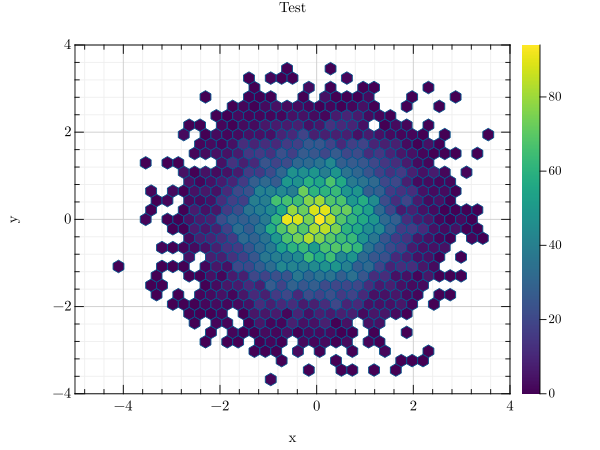
Following parameters can be used: cmap, columns, consecutive_colorbars, file, grplot, ignore_blank_lines, join_plots, keep_aspect_ratio, kind, only_square_aspect_ratio, resample_method, title, use_bins, x_columns, x_flip, x_grid, x_label, x_lim, x_log, x_range, xyz_file, y_columns, y_flip, y_grid, y_label, y_lim, y_log, y_range, z_lim, z_log, z_range hexbin¶A hexbin uses hexagonal binning and the current colour map to display the data. Such a plot can be easily created from the command line using the following command: grplot hexbin.dat kind:hexin This example uses the hexbin data file. It contains additional key-value pairs in the data header. More information’s about the format of these files can be found under data_file. # title : Test # x_label : x # y_label : y
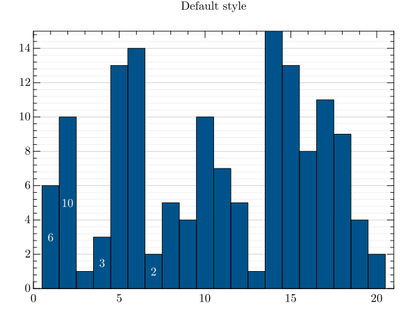
Following parameters can be used: cmap, columns, consecutive_colorbars, file, grplot, ignore_blank_lines, join_plots, keep_aspect_ratio, kind, num_bins, only_square_aspect_ratio, title, x_columns, x_flip, x_grid, x_label, x_lim, x_range, y_columns, y_flip, y_grid, y_label, y_lim, y_range histogram¶A histogram provides an approximate representation of the distribution of numerical data. It should have two columns
containing the x- and y-data. To create a histogram from the command line, use grplot histogram.dat kind:histogram num_bins:20 In the right plot, these parameters are extended to include a vertical orientation with # x_range : 2,3 # y_range : 5, 8
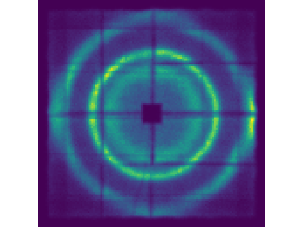
Following parameters can be used: bar_color, bottom, columns, edge_color, error, error_bar_style, error_columns, error_type, equal_up_and_down_error, file, grplot, ignore_blank_lines, join_plots, keep_aspect_ratio, kind, left, num_bins, orientation, right, title, top, twin_x, twin_y, x_grid, x_label, x_lim, x_log, x_range, xye_file, y_columns, y_flip, y_grid, y_label, y_lim, y_log imshow¶An imshow plot displays data as a coloured image, with each data point represented by a coloured rectangle within the
image. To create an imshow plot from the command line, grplot sans.dat kind:imshow
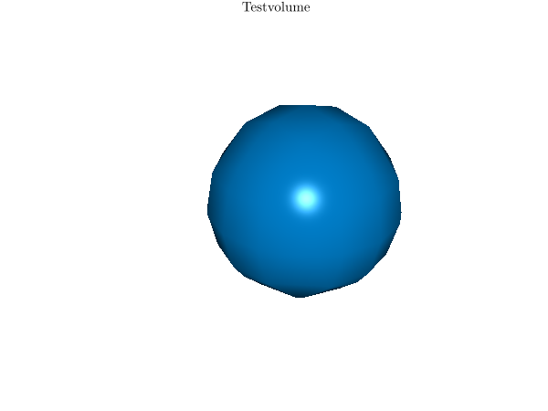
Following parameters can be used: cmap, columns, file, grplot, ignore_blank_lines, keep_aspect_ratio, kind, only_square_aspect_ratio, title, x_columns, x_flip, xyz_file, y_columns, y_flip, z_lim isosurface¶An isosurface is a three-dimensional analogue of a contour- or isoline. To create an isosurface from the command line,
the grplot volume.dat kind:isosurface
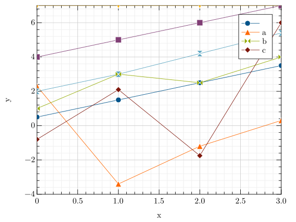
Following parameters can be used: columns, file, grplot, ignore_blank_lines, isovalue, join_plots, kind, rotation, tilt, title, x_columns, x_flip, x_lim, x_log, x_range, xyz_file, y_columns, y_flip, y_lim, y_log, y_range, z_grid, z_lim, z_log, z_range line¶A line plot is a simple graph in which data points are joined together by a line. To create a line plot from the command
line, the grplot covid19.csv kind:line The following example includes parameters defined in the data header, such as the title and axis labels. The parameter
# title : Confirmed SARS–CoV–2 infections
# x_label : Day
# y_label : Confirmed
# x_lim : 0.0, 917 + 1.0
# y_log : 1
# location : 4
The right-hand plot uses command-line arguments and the target_mtl data file. grplot target_mtl.1D kind:line y_log:1
A line plot can be combined with a scatter plot to mark data points. The grplot stem.dat kind:line line_spec:+-
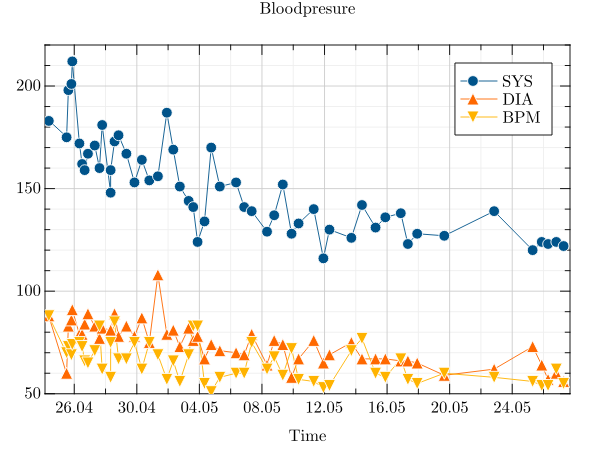
Another common use of a line plot is to display time data. For these GRPlot applies some defaults such as
grplot blood_pressure.csv
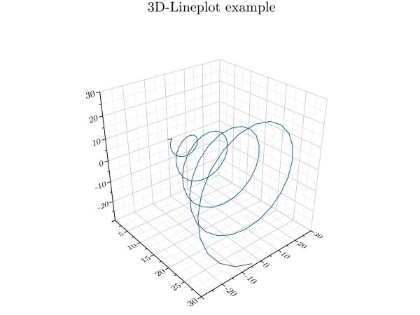
Following parameters can be used: bottom, columns, error, error_bar_style, error_columns, error_type, equal_up_and_down_error, file, grplot, ignore_blank_lines, int_limits_high, int_limits_low, join_plots, keep_aspect_ratio, kind, left, legend, legend_line, line_spec, location, marker_size, marker_type, orientation, right, title, top, twin_x, twin_y, x_columns, x_flip, x_grid, x_label, x_lim, x_log, x_range, xye_file, y_columns, y_flip, y_grid, y_label, y_lim, y_log, y_range line3¶A line3 plot is a simple three-dimensional graph in which data points are joined together by a line. To create a
three-dimensional line plot from the command line, the grplot plot3.dat kind:line3
Following parameters can be used: columns, file, grplot, hkind, ignore_blank_lines, join_plots, kind, legend, legend_line, location, title, x_columns, x_flip, x_grid, x_label, x_lim, x_log, x_range, xyz_file, y_columns, y_flip, y_grid, y_label, y_lim, y_log, y_range, z_grid, z_label, z_lim, z_log, z_range marginal_heatmap¶A marginal heatmap combines a heatmap with either stair plots or histograms. These additional plots display some of the
heatmap data in the vertical and horizontal directions at the margins of the heatmap. To create a marginal heatmap from
the command line, use grplot sans.dat kind:marginal_heatmap When grplot sample_y_divy.dat kind:marginal_heatmap use_bins:1 h_kind:line
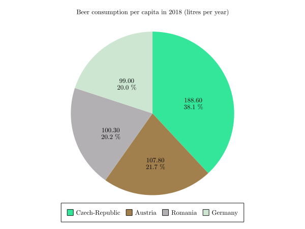
Following parameters can be used: algorithm, cmap, columns, file, grplot, hkind, ignore_blank_lines, join_plots, keep_aspect_ratio, kind, only_square_aspect_ratio, resample_method, title, use_bins, x_columns, x_flip, x_grid, x_label, x_lim, x_log, x_range, xyz_file, y_columns, y_flip, y_grid, y_label, y_lim, y_log, y_range, z_lim, z_log, z_range pie¶A pie chart is a circular statistical plot that displays one series of data. The total area of the chart represents the
total percentage of the given data. The size of each slice represents the percentage of the data it comprises. To create
a pie chart from the command line, the grplot pie.dat kind:pie
Following parameters can be used: columns, file, grplot, ignore_blank_lines, kind, legend, legend_line, title polar_heatmap¶A polar heatmap uses polar coordinates rather than Cartesian coordinates. To create a polar heatmap plot from the
command line, the grplot polarheatmap.dat kind:polar_heatmap With an additional
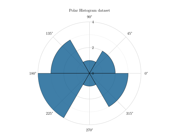
Following parameters can be used: cmap, columns, consecutive_colorbars, file, grplot, ignore_blank_lines, join_plots, kind, r_flip, r_lim, r_log, theta_flip, theta_data_lim, theta_lim, title, x_columns, x_label, y_columns, y_label polar_histogram¶A polar histogram is a histogram that uses polar coordinates. To create a polar histogram plot from the command line,
set the grplot polar_histogram.dat kind:polar_histogram
Additional parameters offer more possibilities such as r_lim:2,8 keep_radii_axes:1
or stairs:1
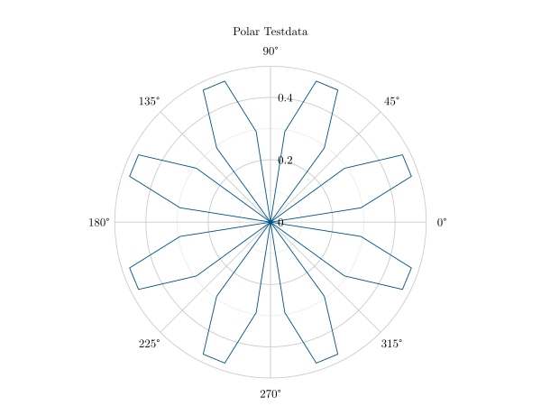
Following parameters can be used: bin_counts, bin_edges, bin_width, columns, draw_edges, edge_color, file, grplot, ignore_blank_lines, join_plots, keep_radii_axes, kind, num_bins, normalization, r_flip, r_lim, r_log, stairs, theta_flip, theta_data_lim, theta_lim, title, x_columns, x_label, y_columns, y_label polar_line¶A polar plot displays a polyline in polar coordinates. The angle in radians is indicated by theta(x), and the radius
value for each point is indicated by r(y). To create a polar line plot from the command line, the grplot polar.dat kind:polar_line
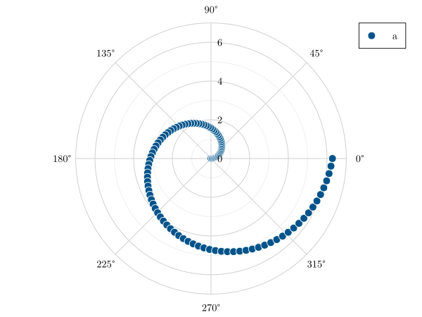
Following parameters can be used: clip_negative, columns, file, grplot, ignore_blank_lines, join_plots, kind, legend, legend_line, line_spec, location, marker_size, marker_type, r_flip, r_lim, r_log, theta_flip, theta_data_lim, theta_lim, title, x_columns, x_label, y_columns, y_label polar_scatter¶In a polar scatter plot, each data point is displayed as a point within a polar coordinate system. Theta(x) indicates
the angle in radians and r(y) indicates the radius for each point. To create a polar scatter plot from the command line,
the grplot polar_thetatheta.dat kind:polar_scatter
Following parameters can be used: clip_negative, columns, file, grplot, ignore_blank_lines, join_plots, kind, legend, legend_line, line_spec, location, marker_size, marker_type, r_flip, r_lim, r_log, theta_flip, theta_data_lim, theta_lim, title, x_columns, x_label, y_columns, y_label scatter¶In a scatter plot, each data point is displayed as an individual point within a two-dimensional coordinate system. A
scatter plot can be created from the command line using the grplot scatter.dat kind:scatter marker_type:-7 If there are multiple series, each scatter plot gets its own marker. The grplot target_mtl.1D kind:scatter y_log:1 columns:1,2,3
Following parameters can be used: bottom, columns, file, grplot, ignore_blank_lines, join_plots, keep_aspect_ratio, kind, left, legend, legend_line, line_spec, location, marker_size, marker_type, orientation, right, title, top, twin_x, twin_y, x_columns, x_flip, x_grid, x_label, x_lim, x_log, x_range, xye_file, y_columns, y_flip, y_grid, y_label, y_lim, y_log, y_range scatter3¶A three-dimensional scatter plot shows each data point as an individual point within a three-dimensional coordinate
system. To create a 3d scatter plot from the command line, set the kind parameter to grplot plot3.dat kind:scatter3 A colored 3d scatter plot can be created by defining additional color values (
Following parameters can be used: columns, file, grplot, ignore_blank_lines, join_plots, kind, legend, legend_line, location, title, x_columns, x_flip, x_grid, x_label, x_lim, x_log, x_range, xyz_file, y_columns, y_flip, y_grid, y_label, y_lim, y_log, y_range, z_grid, z_label, z_lim, z_log, z_range shade¶A shade plot can be used to create a heatmap from point- or line-based data. To create a shade plot using GRPlot, set
the plot type to grplot hexbin.dat kind:shade The additional x- and y-bins parameters define the number of bins in each direction, while a cubic transformation is also used for the right-hand image. Combining these additional parameters helps to produce a more meaningful result. grplot hexbin.dat kind:shade x_bins:50 y_bins:50 transformation:4
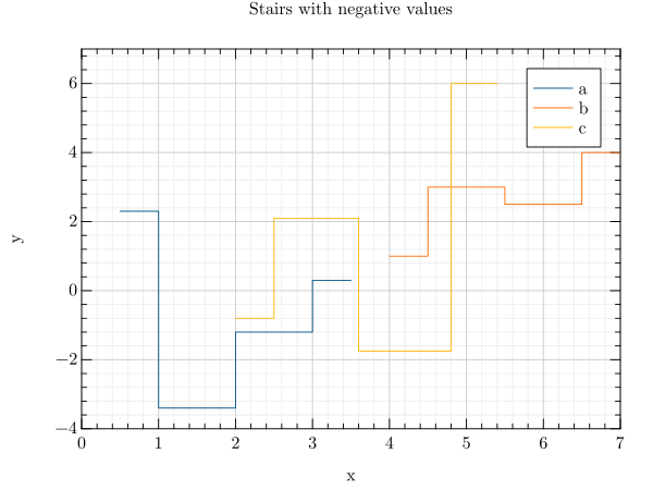
Following parameters can be used: cmap, columns, file, grplot, ignore_blank_lines, join_plots, keep_aspect_ratio, kind, only_square_aspect_ratio, transformation, x_bins, x_flip, x_grid, x_label, x_lim, x_log, x_range, y_bins, y_flip, y_grid, y_label, y_lim, y_log, y_range, z_lim, z_log, z_range stairs¶A stair plot is a piecewise constant function with a finite number of pieces. To create a stair plot from the command
line, use the grplot stem.dat kind:stairs
Following parameters can be used: bottom, columns, file, grplot, ignore_blank_lines, join_plots, keep_aspect_ratio, kind, left, legend, legend_line, line_spec, location, marker_type, orientation, right, step_where, title, top, twin_x, twin_y, x_columns, x_flip, x_grid, x_label, x_lim, x_log, x_range, y_columns, y_flip, y_grid, y_label, y_lim, y_log, y_range stem¶In a stem plot, lines are drawn perpendicular to the baseline at each point between the baseline and the data values. To
create a stem plot from the command line, use grplot stem.dat kind:stem x_columns:1,4,6 y_columns:2,5,7
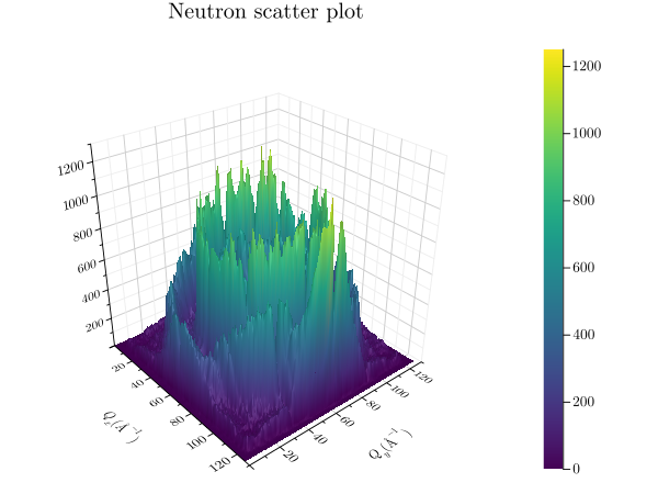
Following parameters can be used: bottom, columns, file, grplot, ignore_blank_lines, join_plots, keep_aspect_ratio, kind, left, legend, legend_line, location, marker_type, orientation, right, title, top, twin_x, twin_y, x_columns, x_flip, x_grid, x_label, x_lim, x_log, x_range, y_columns, y_flip, y_grid, y_label, y_lim, y_log, y_range surface¶A surface plot can be compared with a visualisation of a two-variable function in three-dimensional space. To create a
surface plot from the command line, the grplot sans.dat kind:surface
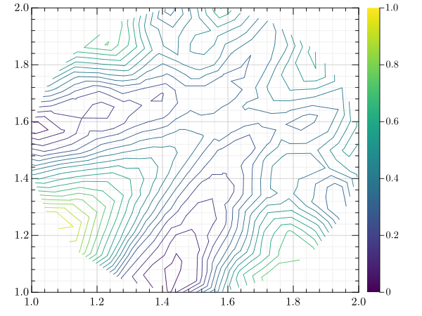
Following parameters can be used: accelerate, cmap, columns, consecutive_colorbars, file, grplot, ignore_blank_lines, join_plots, kind, use_bins, x_columns, x_flip, x_grid, x_label, x_lim, x_log, x_range, xyz_file, y_columns, y_flip, y_grid, y_label, y_lim, y_log, y_range, z_grid, z_label, z_lim, z_log, z_range tricontour¶A tricontour plot shows contour lines on an unstructured triangular grid. To create a tricontour plot from the command
line, set the grplot tricontour.dat kind:tricontour
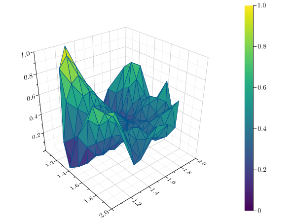
Following parameters can be used: cmap, columns, consecutive_colorbars, file, grplot, ignore_blank_lines, join_plots, keep_aspect_ratio, kind, levels, x_columns, x_flip, x_grid, x_label, x_lim, x_log, x_range, xyz_file, y_columns, y_flip, y_grid, y_label, y_lim, y_log, y_range, z_lim, z_log, z_range trisurface¶A trisurface is a type of surface plot created by triangulating compact surfaces consisting of a finite number of
triangles that cover the entire surface, ensuring that each point on the surface lies within a triangle. To create a
trisurface plot from the command line, the grplot tricontour.dat kind:trisurface
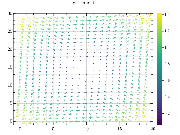
Following parameters can be used: cmap, columns, consecutive_colorbars, file, grplot, ignore_blank_lines, join_plots, kind, x_columns, x_flip, x_grid, x_label, x_lim, x_log, x_range, xyz_file, y_columns, y_flip, y_grid, y_label, y_lim, y_log, y_range, z_grid, z_label, z_lim, z_log, z_range quiver¶A quiver plot is a type of two-dimensional plot that displays vectors as arrows. To create a quiver plot from the
command line, the grplot quiver.dat kind:quiver
Following parameters can be used: cmap, columns, consecutive_colorbars, file, grplot, hkind, ignore_blank_lines, join_plots, keep_aspect_ratio, kind, title, x_flip, x_grid, x_label, x_lim, x_log, x_range, y_flip, y_grid, y_label, y_lim, y_log, y_range, z_lim volume¶A volume plot uses volume rendering to draw a three-dimensional data set. The volume data is first reduced to a
two-dimensional image using either an emission or an absorption model, or via a maximum intensity projection. The
current colormap is then applied to the result. To create a volume plot from the command line, the grplot volume.dat kind:volume algorithm:emission
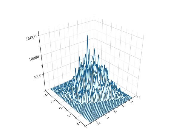
Following parameters can be used: algorithm, cmap, columns, consecutive_colorbars, file, grplot, ignore_blank_lines, join_plots, kind, title, x_columns, x_flip, x_grid, x_label, x_lim, x_log, x_range, y_columns, y_flip, y_grid, y_label, y_lim, y_log, y_range, z_grid, z_label, z_lim, z_log, z_range wireframe¶In a wireframe plot, a grid of values is projected onto a specified three-dimensional surface. This surface has a grid
structure itself. To create a wireframe plot from the command line, the grplot sample_y_divy.dat kind:wireframe use_bins:1
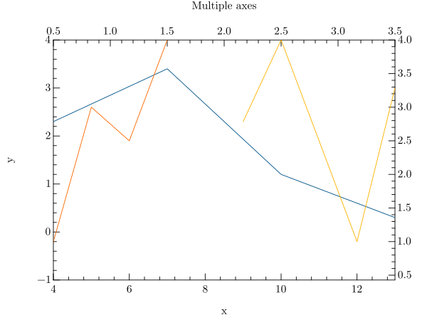
Following parameters can be used: columns, file, grplot, ignore_blank_lines, join_plots, kind, use_bins, x_columns, x_flip, x_grid, x_label, x_lim, x_log, x_range, xyz_file, y_columns, y_flip, y_grid, y_label, y_lim, y_log, y_range, z_grid, z_label, z_lim, z_log, z_range Multiple axes¶To create a plot with additional axes, the multi_axes.dat x_columns:1,4,6 y_columns:2,5,7 twin_x:0 twin_y:1 kind:line
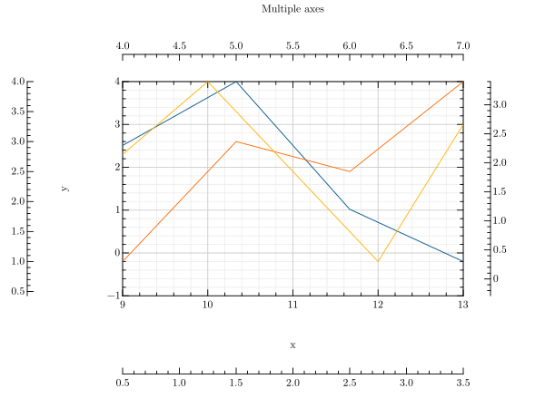
Another example that uses twin axes is: multi_axes.dat x_columns:1,4,6 y_columns:2,5,7 right:0 left:1 bottom:0 top:1 kind:line
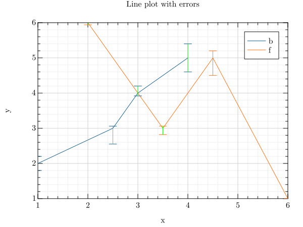
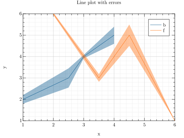
Following parameters can be useful for it: Error bars¶There are multiple ways to display error data. For example, you can use grplot line_error.dat kind:line error:{error_bar_color:3} x_columns:1,5 y_columns:2,6 error_columns:3,4,7,8
The style of the error bars can be changed too. grplot line_error.dat kind:line x_columns:1,5 y_columns:2,6 error_columns:3,7 error_bar_style:1 equal_up_and_down_error:1
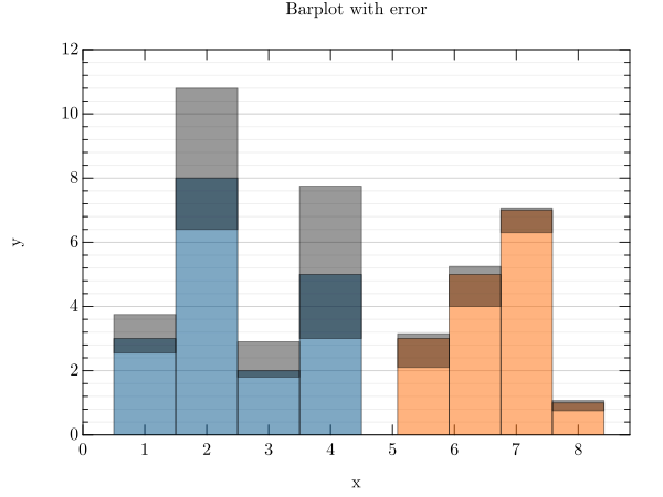
In the case of a bar plot, the key value pair grplot barplot_error.dat kind:barplot bar_width:1 error_bar_style:1 x_columns:1,3 y_columns:2,4 error_columns:5,6,7,8 error:{} y_lim:0,12
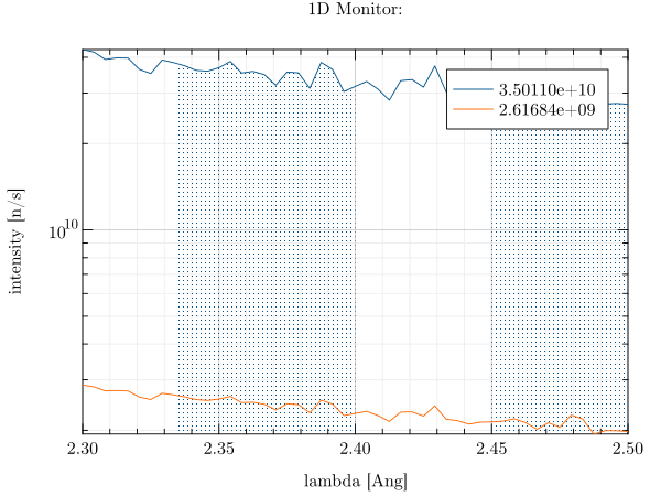
Following parameters can be useful for it: error, error_bar_style, error_columns, error_type, equal_up_and_down_error, xye_file Integral¶An integral can be created for line plots using the grplot lambda.dat kind:line int_limits_high:2,2.4,2.5 int_limits_low:2,2.335,2.45 columns:2,3 y_log:1
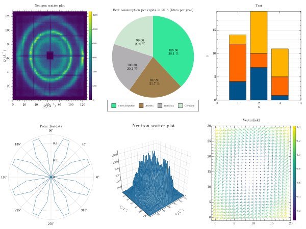
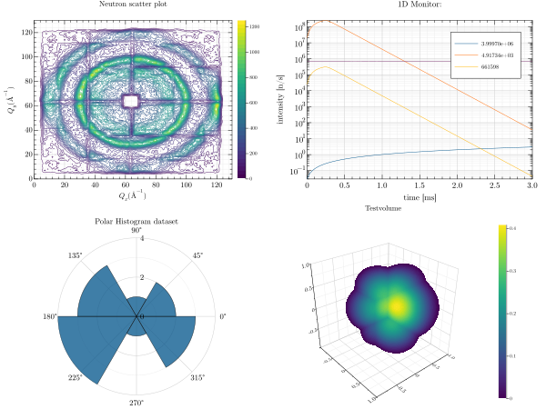
Following parameters can be useful for it: Multiplot¶To create multiple plots, it is necessary to use the grplot \ --plot ./lib/grm/grplot/data/sans.dat kind:heatmap \ --plot ./lib/grm/grplot/data/polar.dat kind:polar_line \ --plot ./lib/grm/grplot/data/pie.dat kind:pie \ --plot ./lib/grm/grplot/data/sans.dat kind:wireframe \ --plot ./lib/grm/grplot/data/barplot.dat kind:barplot style:stacked \ --plot ./lib/grm/grplot/data/quiver.dat kind:quiver
grplot \
  --plot ./lib/grm/grplot/data/sans.dat kind:contour levels:40 \
  --plot ./lib/grm/grplot/data/polar_histogram.dat kind:polar_histogram \
  --plot ./lib/grm/grplot/data/source_time.dat kind:line y_log:1 \
  --plot ./lib/grm/grplot/data/volume.dat kind:volume
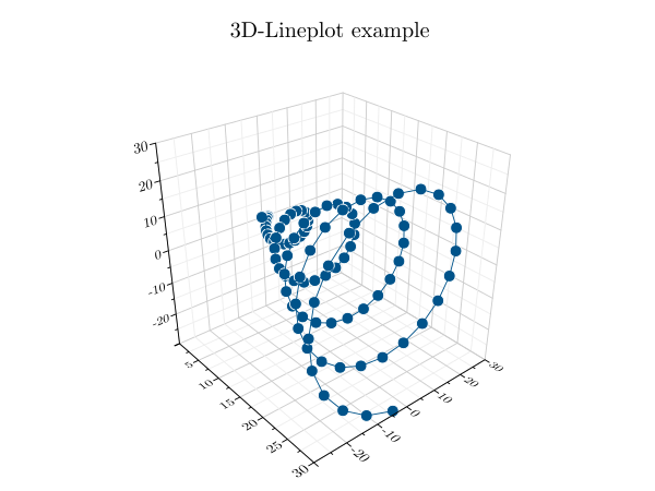
The editor must be used to apply larger changes, such as adding multiple columns or rows to a single plot. Mixed plots¶Similar to the multi plots, a mixed plot of different series can be created. To do this, the grplot \ --plot ./lib/grm/grplot/data/plot3.dat kind:scatter3 \ --plot ./lib/grm/grplot/data/plot3.dat kind:line3 join_plots:1,2
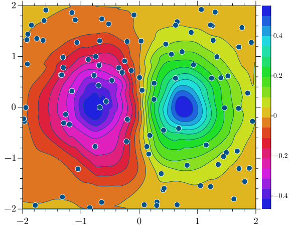
Another example, which uses a combination of a scatter and a contour plot, can be created with this command line inside GRPlot. This example is also used in other places in this documentation. This one uses the mixed_series and mixed_series_contour dataset. grplot \ --plot ./lib/grm/grplot/data/mixed_series_contour.dat kind:contourf x_range:-2,2 y_range:-2,2 colormap:48 \ --plot ./lib/grm/grplot/data/mixed_series.dat kind:scatter x_columns:1 y_columns:2 columns:1,2 join_plots:1,2
Following parameters can be useful for it: Colorbar¶There are three main ways to modify the colorbar inside GRPlot. One option is to change the colormap, while another is to adjust the location of the colorbar, which can be quickly changed between four locations.
The third option is to adjust the limits that the colour bar displays. In a multiplot, all colorbars can easily be
modified to have the same limits. To do this, the
This last example was created using a trick that alters the z-value ranges, giving the grplot \ --plot ./lib/grm/grplot/data/sample_y_divy.dat kind:heatmap use_bins:1 z_range:-20000,80000 \ --plot ./lib/grm/grplot/data/sample.dat kind:heatmap use_bins:1 y_lim:-0.25,0.25 Following parameters can be useful for it: |
| You are visitor 01402503 — GeezerVison does not store the pages you look up. Best viewed with Netscape Navigator 4.7 or Internet Explorer 6 at 800×600. No cookies required. |