Python Data Structure - Quick Guide

---

---

Python - DS Introduction

Here, we will understand what is data structure with regards to Python programming language.

Data Structure Overview

Data structures are fundamental concepts of computer science which helps is writing efficient programs in any language. Python is a high-level, interpreted, interactive and object-oriented scripting language using which we can study the fundamentals of data structure in a simpler way as compared to other programming languages.

In this chapter we are going to study a short overview of some frequently used data structures in general and how they are related to some specific python data types. There are also some data structures specific to python which is listed as another category.

General Data Structures

The various data structures in computer science are divided broadly into two categories shown below. We will discuss about each of the below data structures in detail in subsequent chapters.

Liner Data Structures

These are the data structures which store the data elements in a sequential manner.

• Array − It is a sequential arrangement of data elements paired with the index of the data element.

• Linked List − Each data element contains a link to another element along with the data present in it.

• Stack − It is a data structure which follows only to specific order of operation. LIFO(last in First Out) or FILO(First in Last Out).

• Queue − It is similar to Stack but the order of operation is only FIFO(First In First Out).

• Matrix − It is two dimensional data structure in which the data element is referred by a pair of indices.

Non-Liner Data Structures

These are the data structures in which there is no sequential linking of data elements. Any pair or group of data elements can be linked to each other and can be accessed without a strict sequence.

• Binary Tree − It is a data structure where each data element can be connected to maximum two other data elements and it starts with a root node.

• Heap − It is a special case of Tree data structure where the data in the parent node is either strictly greater than/ equal to the child nodes or strictly less than its child nodes.

• Hash Table − It is a data structure which is made of arrays associated with each other using a hash function. It retrieves values using keys rather than index from a data element.

• Graph − It is an arrangement of vertices and nodes where some of the nodes are connected to each other through links.

Python Specific Data Structures

These data structures are specific to python language and they give greater flexibility in storing different types of data and faster processing in python environment.

• List − It is similar to array with the exception that the data elements can be of different data types. You can have both numeric and string data in a python list.

• Tuple − Tuples are similar to lists but they are immutable which means the values in a tuple cannot be modified they can only be read.

• Dictionary − The dictionary contains Key-value pairs as its data elements.

In the next chapters we are going to learn the details of how each of these data structures can be implemented using Python.

Python - DS Environment

Python is available on a wide variety of platforms including Linux and Mac OS X. Let's understand how to set up our Python environment.

Local Environment Setup

Open a terminal window and type "python" to find out if it is already installed and which version is installed.

• Unix (Solaris, Linux, FreeBSD, AIX, HP/UX, SunOS, IRIX, etc.)
• Win 9x/NT/2000
• Macintosh (Intel, PPC, 68K)
• OS/2
• DOS (multiple versions)
• PalmOS
• Nokia mobile phones
• Windows CE
• Acorn/RISC OS
• BeOS
• Amiga
• VMS/OpenVMS
• QNX
• VxWorks
• Psion
• Python has also been ported to the Java and .NET virtual machines

Getting Python

The most up-to-date and current source code, binaries, documentation, news, etc., is available on the official website of Python www.python.org

You can download Python documentation from this website given herewith,www.python.org/doc. The documentation is available in HTML, PDF, and PostScript formats.

Installing Python

Python distribution is available for a wide variety of platforms. You need to download only the binary code applicable for your platform and install Python.

If the binary code for your platform is not available, you need a C compiler to compile the source code manually. Compiling the source code offers more flexibility in terms of choice of features that you require in your installation.

Here is a quick overview of installing Python on various platforms −

Unix and Linux Installation

Here are the simple steps to install Python on Unix/Linux machine.

• Open a Web browser and go to www.python.org/downloads.

• Follow the link to download zipped source code available for Unix/Linux.

• Download and extract files.

• Editing the Modules/Setup file if you want to customize some options.

• run ./configure script

• make

• make install

This installs Python at standard location /usr/local/bin and its libraries at /usr/local/lib/pythonXX where XX is the version of Python.

Windows Installation

Here are the steps to install Python on Windows machine.

• Open a Web browser and go to www.python.org/downloads.

• Follow the link for the Windows installer python-XYZ.msi file where XYZ is the version you need to install.

• To use this installer python-XYZ.msi, the Windows system must support Microsoft Installer 2.0. Save the installer file to your local machine and then run it to find out if your machine supports MSI.

• Run the downloaded file. This brings up the Python install wizard, which is really easy to use. Just accept the default settings, wait until the install is finished, and you are done.

Macintosh Installation

Recent Macs come with Python installed, but it may be several years out of date. See www.python.org/download/mac/ for instructions on getting the current version along with extra tools to support development on the Mac. For older Mac OS's before Mac OS X 10.3 (released in 2003), MacPython is available.

Jack Jansen maintains it and you can have full access to the entire documentation at his website − https://homepages.cwi.nl/~jack/macpython/index.html. You can find complete installation details for Mac OS installation.

Setting up PATH

Programs and other executable files can be in many directories, so operating systems provide a search path that lists the directories that the OS searches for executables.

The path is stored in an environment variable, which is a named string maintained by the operating system. This variable contains information available to the command shell and other programs.

The path variable is named as PATH in Unix or Path in Windows (Unix is case sensitive; Windows is not).

In Mac OS, the installer handles the path details. To invoke the Python interpreter from any particular directory, you must add the Python directory to your path.

Setting path at Unix/Linux

To add the Python directory to the path for a particular session in Unix −

• In the csh shell − type setenv PATH "$PATH:/usr/local/bin/python" and press Enter.

• In the bash shell (Linux) − type export ATH="$PATH:/usr/local/bin/python" and press Enter.

• In the sh or ksh shell − type PATH="$PATH:/usr/local/bin/python" and press Enter.

• Note − /usr/local/bin/python is the path of the Python directory

Setting path at Windows

To add the Python directory to the path for a particular session in Windows −

• At the command prompt − type path %path%;C:\Python and press Enter.

• Note − C:\Python is the path of the Python directory

Python Environment Variables

Here are important environment variables, which can be recognized by Python −

Running Python

There are three different ways to start Python, which are as follows −

Interactive Interpreter

• You can start Python from Unix, DOS, or any other system that provides you a command-line interpreter or shell window.

• Enter python the command line.

• Start coding right away in the interactive interpreter.

$python # Unix/Linux
or
python% # Unix/Linux
or
C:> python # Windows/DOS

Here is the list of all the available command line options, which is as mentioned below −

Script from the Command-line

A Python script can be executed at command line by invoking the interpreter on your application, as in the following −

$python script.py # Unix/Linux

or

python% script.py # Unix/Linux

or 

C: >python script.py # Windows/DOS

• Note − Be sure the file permission mode allows execution.

Integrated Development Environment(IDE)

You can run Python from a Graphical User Interface (GUI) environment as well, if you have a GUI application on your system that supports Python.

• Unix − IDLE is the very first Unix IDE for Python.

• Windows − PythonWin is the first Windows interface for Python and is an IDE with a GUI.

• Macintosh − The Macintosh version of Python along with the IDLE IDE is available from the main website, downloadable as either MacBinary or BinHex'd files.

If you are not able to set up the environment properly, then you can take help from your system admin. Make sure the Python environment is properly set up and working perfectly fine.

• Note − All the examples given in subsequent chapters are executed with Python 2.4.3 version available on CentOS flavor of Linux.

We already have set up Python Programming environment online, so that you can execute all the available examples online at the same time when you are learning theory. Feel free to modify any example and execute it online.

Python - Arrays

Array is a container which can hold a fix number of items and these items should be of the same type. Most of the data structures make use of arrays to implement their algorithms. Following are the important terms to understand the concept of Array are as follows −

• Element − Each item stored in an array is called an element.

• Index − Each location of an element in an array has a numerical index, which is used to identify the element.

Array Representation

Arrays can be declared in various ways in different languages. Below is an illustration.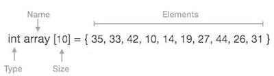

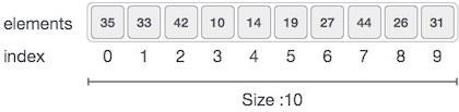
As per the above illustration, following are the important points to be considered −

• Index starts with 0.

• Array length is 10, which means it can store 10 elements.

• Each element can be accessed via its index. For example, we can fetch an element at index 6 as 9.

Basic Operations

The basic operations supported by an array are as stated below −

• Traverse − print all the array elements one by one.

• Insertion − Adds an element at the given index.

• Deletion − Deletes an element at the given index.

• Search − Searches an element using the given index or by the value.

• Update − Updates an element at the given index.

Array is created in Python by importing array module to the python program. Then, the array is declared as shown below −

from array import *

arrayName = array(typecode, [Initializers])

Typecode are the codes that are used to define the type of value the array will hold. Some common typecodes used are as follows −

Before looking at various array operations lets create and print an array using python.

Example

The below code creates an array named array1.

from array import *

array1 = array('i', [10,20,30,40,50])

for x in array1:
   print(x)

Output

When we compile and execute the above program, it produces the following result −

10
20
30
40
50

Accessing Array Element

We can access each element of an array using the index of the element. The below code shows how to access an array element.

Example

from array import *

array1 = array('i', [10,20,30,40,50])

print (array1[0])

print (array1[2])

Output

When we compile and execute the above program, it produces the following result, which shows the element is inserted at index position 1.

10
30

Insertion Operation

Insert operation is to insert one or more data elements into an array. Based on the requirement, a new element can be added at the beginning, end, or any given index of array.

Example

Here, we add a data element at the middle of the array using the python in-built insert() method.

from array import *

array1 = array('i', [10,20,30,40,50])

array1.insert(1,60)

for x in array1:
   print(x)

When we compile and execute the above program, it produces the following result which shows the element is inserted at index position 1.

Output

10
60
20
30
40
50

Deletion Operation

Deletion refers to removing an existing element from the array and re-organizing all elements of an array.

Example

Here, we remove a data element at the middle of the array using the python in-built remove() method.

from array import *

array1 = array('i', [10,20,30,40,50])

array1.remove(40)

for x in array1:
   print(x)

Output

When we compile and execute the above program, it produces the following result which shows the element is removed form the array.

10
20
30
50

Search Operation

You can perform a search for an array element based on its value or its index.

Example

Here, we search a data element using the python in-built index() method.

from array import *

array1 = array('i', [10,20,30,40,50])

print (array1.index(40))

Output

When we compile and execute the above program, it produces the following result which shows the index of the element. If the value is not present in the array then th eprogram returns an error.

3

Update Operation

Update operation refers to updating an existing element from the array at a given index.

Example

Here, we simply reassign a new value to the desired index we want to update.

from array import *

array1 = array('i', [10,20,30,40,50])

array1[2] = 80

for x in array1:
   print(x)

Output

When we compile and execute the above program, it produces the following result which shows the new value at the index position 2.

10
20
80
40
50

Python - Lists

The list is a most versatile datatype available in Python which can be written as a list of comma-separated values (items) between square brackets. Important thing about a list is that items in a list need not be of the same type.

Creating a list is as simple as putting different comma-separated values between square brackets.

For example

list1 = ['physics', 'chemistry', 1997, 2000]
list2 = [1, 2, 3, 4, 5 ]
list3 = ["a", "b", "c", "d"]

Similar to string indices, list indices start at 0, and lists can be sliced, concatenated and so on.

Accessing Values

To access values in lists, use the square brackets for slicing along with the index or indices to obtain value available at that index.

For example

#!/usr/bin/python

list1 = ['physics', 'chemistry', 1997, 2000]
list2 = [1, 2, 3, 4, 5, 6, 7 ]
print ("list1[0]: ", list1[0])
print ("list2[1:5]: ", list2[1:5])

When the above code is executed, it produces the following result −

list1[0]:  physics
list2[1:5]:  [2, 3, 4, 5]

Updating Lists

You can update single or multiple elements of lists by giving the slice on the left-hand side of the assignment operator, and you can add to elements in a list with the append() method.

For example

#!/usr/bin/python

list = ['physics', 'chemistry', 1997, 2000]
print ("Value available at index 2 : ")
print (list[2])
list[2] = 2001
print ("New value available at index 2 : ")
print (list[2])

• Note − append() method is discussed in subsequent section.

When the above code is executed, it produces the following result −

Value available at index 2 :
1997
New value available at index 2 :
2001

Delete List Elements

To remove a list element, you can use either the del statement if you know exactly which element(s) you are deleting or the remove() method if you do not know.

For example

#!/usr/bin/python

list1 = ['physics', 'chemistry', 1997, 2000]
print (list1)
del list1[2]
print ("After deleting value at index 2 : ")
print (list1)

When the above code is executed, it produces following result −

['physics', 'chemistry', 1997, 2000]
After deleting value at index 2 :
['physics', 'chemistry', 2000]

• Note − remove() method is discussed in subsequent section.

Basic List Operations

Lists respond to the + and * operators much like strings; they mean concatenation and repetition here too, except that the result is a new list, not a string.

In fact, lists respond to all of the general sequence operations we used on strings in the prior chapter.

Python - Tuples

A tuple is a sequence of immutable Python objects. Tuples are sequences, just like lists. The differences between tuples and lists are, the tuples cannot be changed unlike lists and tuples use parentheses, whereas lists use square brackets.

Creating a tuple is as simple as putting different comma-separated values. Optionally you can put these comma-separated values between parentheses also.

For example

tup1 = ('physics', 'chemistry', 1997, 2000);
tup2 = (1, 2, 3, 4, 5 );
tup3 = "a", "b", "c", "d";

The empty tuple is written as two parentheses containing nothing −

tup1 = ();

To write a tuple containing a single value you have to include a comma, even though there is only one value −

tup1 = (50,);

Like string indices, tuple indices start at 0, and they can be sliced, concatenated, and so on.

Accessing Values in Tuples

To access values in tuple, use the square brackets for slicing along with the index or indices to obtain value available at that index.

For example

#!/usr/bin/python

tup1 = ('physics', 'chemistry', 1997, 2000);
tup2 = (1, 2, 3, 4, 5, 6, 7 );
print ("tup1[0]: ", tup1[0])
print ("tup2[1:5]: ", tup2[1:5])

When the above code is executed, it produces the following result −

tup1[0]:  physics
tup2[1:5]:  [2, 3, 4, 5]

Updating Tuples

Tuples are immutable which means you cannot update or change the values of tuple elements. You are able to take portions of existing tuples to create new tuples as the following example demonstrates −

#!/usr/bin/python

tup1 = (12, 34.56);
tup2 = ('abc', 'xyz');

# Following action is not valid for tuples
# tup1[0] = 100;

# So let's create a new tuple as follows
tup3 = tup1 + tup2;
print (tup3);

When the above code is executed, it produces the following result −

(12, 34.56, 'abc', 'xyz')

Delete Tuple Elements

Removing individual tuple elements is not possible. There is, of course, nothing wrong with putting together another tuple with the undesired elements discarded.

To explicitly remove an entire tuple, just use the del statement.

For example

#!/usr/bin/python

tup = ('physics', 'chemistry', 1997, 2000);
print (tup);
del tup;
print ("After deleting tup : ");
print (tup);

• Note − an exception raised, this is because after del tup tuple does not exist anymore.

This produces the following result −

('physics', 'chemistry', 1997, 2000)
After deleting tup :
Traceback (most recent call last):
   File "test.py", line 9, in <module>
      print tup;
NameError: name 'tup' is not defined

Basic Tuples Operations

Tuples respond to the + and * operators much like strings; they mean concatenation and repetition here too, except that the result is a new tuple, not a string.

In fact, tuples respond to all of the general sequence operations we used on strings in the prior chapter.

Python - Dictionary

In Dictionary each key is separated from its value by a colon (:), the items are separated by commas, and the whole thing is enclosed in curly braces. An empty dictionary without any items is written with just two curly braces, like this − {}.

Keys are unique within a dictionary while values may not be. The values of a dictionary can be of any type, but the keys must be of an immutable data type such as strings, numbers, or tuples.

Accessing Values in Dictionary

To access dictionary elements, you can use the familiar square brackets along with the key to obtain its value.

Example

A simple example is as follows −

#!/usr/bin/python

dict = {'Name': 'Zara', 'Age': 7, 'Class': 'First'}
print ("dict['Name']: ", dict['Name'])
print ("dict['Age']: ", dict['Age'])

Output

When the above code is executed, it produces the following result −

dict['Name']:  Zara
dict['Age']:  7

If we attempt to access a data item with a key, which is not part of the dictionary, we get an error as follows −

Example

#!/usr/bin/python

dict = {'Name': 'Zara', 'Age': 7, 'Class': 'First'}
print ("dict['Alice']: ", dict['Alice'])

Output

When the above code is executed, it produces the following result −

dict['Alice']:
Traceback (most recent call last):
   File "test.py", line 4, in <module>
      print "dict['Alice']: ", dict['Alice'];
KeyError: 'Alice'

Updating Dictionary

You can update a dictionary by adding a new entry or a key-value pair, modifying an existing entry, or deleting an existing entry as shown below in the simple example −

Example

#!/usr/bin/python

dict = {'Name': 'Zara', 'Age': 7, 'Class': 'First'}
dict['Age'] = 8; # update existing entry
dict['School'] = "DPS School"; # Add new entry

print ("dict['Age']: ", dict['Age'])
print ("dict['School']: ", dict['School'])

Output

When the above code is executed, it produces the following result −

dict['Age']:  8
dict['School']:  DPS School

Delete Dictionary Elements

You can either remove individual dictionary elements or clear the entire contents of a dictionary. You can also delete entire dictionary in a single operation.

Example

To explicitly remove an entire dictionary, just use the del statement. A simple example is as mentioned below −

#!/usr/bin/python

dict = {'Name': 'Zara', 'Age': 7, 'Class': 'First'}
del dict['Name']; # remove entry with key 'Name'
dict.clear();     # remove all entries in dict
del dict ;        # delete entire dictionary

print ("dict['Age']: ", dict['Age'])
print ("dict['School']: ", dict['School'])

• Note −that an exception is raised because after del dict dictionary does not exist any more −

Output

This produces the following result −

dict['Age']:  dict['Age']
dict['School']:  dict['School']

• Note − del() method is discussed in subsequent section.

Properties of Dictionary Keys

Dictionary values have no restrictions. They can be any arbitrary Python object, either standard objects or user-defined objects. However, same is not true for the keys.

There are two important points to remember about dictionary keys −

• More than one entry per key not allowed. Which means no duplicate key is allowed. When duplicate keys encountered during assignment, the last assignment wins.

For example

#!/usr/bin/python

dict = {'Name': 'Zara', 'Age': 7, 'Name': 'Manni'}
print ("dict['Name']: ", dict['Name'])

Output

When the above code is executed, it produces the following result −

dict['Name']:  Manni

Keys must be immutable. Which means you can use strings, numbers or tuples as dictionary keys but something like ['key'] is not allowed.

Example

An example is as follows −

#!/usr/bin/python

dict = {['Name']: 'Zara', 'Age': 7}
print ("dict['Name']: ", dict['Name'])

Output

When the above code is executed, it produces the following result −

Traceback (most recent call last):
   File "test.py", line 3, in <module>
      dict = {['Name']: 'Zara', 'Age': 7};
TypeError: list objects are unhashable

Python - 2-D Array

Two dimensional array is an array within an array. It is an array of arrays. In this type of array the position of an data element is referred by two indices instead of one. So it represents a table with rows an dcolumns of data.

In the below example of a two dimensional array, observer that each array element itself is also an array.

Consider the example of recording temperatures 4 times a day, every day. Some times the recording instrument may be faulty and we fail to record data. Such data for 4 days can be presented as a two dimensional array as below.

Day 1 - 11 12 5 2 
Day 2 - 15 6 10 
Day 3 - 10 8 12 5 
Day 4 - 12 15 8 6 

The above data can be represented as a two dimensional array as below.

T = [[11, 12, 5, 2], [15, 6,10], [10, 8, 12, 5], [12,15,8,6]]

Accessing Values

The data elements in two dimesnional arrays can be accessed using two indices. One index referring to the main or parent array and another index referring to the position of the data element in the inner array.If we mention only one index then the entire inner array is printed for that index position.

Example

The example below illustrates how it works.

from array import *

T = [[11, 12, 5, 2], [15, 6,10], [10, 8, 12, 5], [12,15,8,6]]

print(T[0])

print(T[1][2])

Output

When the above code is executed, it produces the following result −

[11, 12, 5, 2]
10

To print out the entire two dimensional array we can use python for loop as shown below. We use end of line to print out the values in different rows.

Example

from array import *

T = [[11, 12, 5, 2], [15, 6,10], [10, 8, 12, 5], [12,15,8,6]]
for r in T:
   for c in r:
      print(c,end = " ")
   print()

Output

When the above code is executed, it produces the following result −

11 12  5 2 
15  6 10 
10  8 12 5 
12 15  8 6 

Inserting Values

We can insert new data elements at specific position by using the insert() method and specifying the index.

Example

In the below example a new data element is inserted at index position 2.

from array import *
T = [[11, 12, 5, 2], [15, 6,10], [10, 8, 12, 5], [12,15,8,6]]

T.insert(2, [0,5,11,13,6])

for r in T:
   for c in r:
      print(c,end = " ")
   print()

Output

When the above code is executed, it produces the following result −

11 12  5  2 
15  6 10 
 0  5 11 13 6 
10  8 12  5 
12 15  8  6 

Updating Values

We can update the entire inner array or some specific data elements of the inner array by reassigning the values using the array index.

Example

from array import *

T = [[11, 12, 5, 2], [15, 6,10], [10, 8, 12, 5], [12,15,8,6]]

T[2] = [11,9]
T[0][3] = 7
for r in T:
   for c in r:
      print(c,end = " ")
   print()

Output

When the above code is executed, it produces the following result −

11 12 5  7 
15  6 10 
11  9 
12 15 8  6 

Deleting the Values

We can delete the entire inner array or some specific data elements of the inner array by reassigning the values using the del() method with index. But in case you need to remove specific data elements in one of the inner arrays, then use the update process described above.

Example

from array import *
T = [[11, 12, 5, 2], [15, 6,10], [10, 8, 12, 5], [12,15,8,6]]

del T[3]

for r in T:
   for c in r:
      print(c,end = " ")
   print()

Output

When the above code is executed, it produces the following result −

11 12 5 2 
15 6 10 
10 8 12 5 

Python - Matrix

Matrix is a special case of two dimensional array where each data element is of strictly same size. So every matrix is also a two dimensional array but not vice versa.

Matrices are very important data structures for many mathematical and scientific calculations. As we have already discussed two dimnsional array data structure in the previous chapter we will be focusing on data structure operations specific to matrices in this chapter.

We also be using the numpy package for matrix data manipulation.

Matrix Example

Consider the case of recording temprature for 1 week measured in the morning, mid-day, evening and mid-night. It can be presented as a 7X5 matrix using an array and the reshape method available in numpy.

from numpy import * 
a = array([['Mon',18,20,22,17],['Tue',11,18,21,18],
   ['Wed',15,21,20,19],['Thu',11,20,22,21],
   ['Fri',18,17,23,22],['Sat',12,22,20,18],
   ['Sun',13,15,19,16]])
m = reshape(a,(7,5))
print(m)

Output

The above data can be represented as a two dimensional array as below −

[
   ['Mon' '18' '20' '22' '17']
   ['Tue' '11' '18' '21' '18']
   ['Wed' '15' '21' '20' '19']
   ['Thu' '11' '20' '22' '21']
   ['Fri' '18' '17' '23' '22']
   ['Sat' '12' '22' '20' '18']
   ['Sun' '13' '15' '19' '16']
]

Accessing Values

The data elements in a matrix can be accessed by using the indexes. The access method is same as the way data is accessed in Two dimensional array.

Example

from numpy import * 
m = array([['Mon',18,20,22,17],['Tue',11,18,21,18],
   ['Wed',15,21,20,19],['Thu',11,20,22,21],
   ['Fri',18,17,23,22],['Sat',12,22,20,18],
   ['Sun',13,15,19,16]])
    
# Print data for Wednesday
print(m[2])

# Print data for friday evening
print(m[4][3])

Output

When the above code is executed, it produces the following result −

['Wed', 15, 21, 20, 19]
23

Adding a row

Use the below mentioned code to add a row in a matrix.

Example

from numpy import * 
m = array([['Mon',18,20,22,17],['Tue',11,18,21,18],
   ['Wed',15,21,20,19],['Thu',11,20,22,21],
   ['Fri',18,17,23,22],['Sat',12,22,20,18],
   ['Sun',13,15,19,16]])
m_r = append(m,[['Avg',12,15,13,11]],0)

print(m_r)

Output

When the above code is executed, it produces the following result −

[
   ['Mon' '18' '20' '22' '17']
   ['Tue' '11' '18' '21' '18']
   ['Wed' '15' '21' '20' '19']
   ['Thu' '11' '20' '22' '21']
   ['Fri' '18' '17' '23' '22']
   ['Sat' '12' '22' '20' '18']
   ['Sun' '13' '15' '19' '16']
   ['Avg' '12' '15' '13' '11']
]

Adding a column

We can add column to a matrix using the insert() method. here we have to mention the index where we want to add the column and a array containing the new values of the columns added.In the below example we add t a new column at the fifth position from the beginning.

Example

from numpy import * 
m = array([['Mon',18,20,22,17],['Tue',11,18,21,18],
   ['Wed',15,21,20,19],['Thu',11,20,22,21],
   ['Fri',18,17,23,22],['Sat',12,22,20,18],
   ['Sun',13,15,19,16]])
m_c = insert(m,[5],[[1],[2],[3],[4],[5],[6],[7]],1)

print(m_c)

Output

When the above code is executed, it produces the following result −

[
   ['Mon' '18' '20' '22' '17' '1']
   ['Tue' '11' '18' '21' '18' '2']
   ['Wed' '15' '21' '20' '19' '3']
   ['Thu' '11' '20' '22' '21' '4']
   ['Fri' '18' '17' '23' '22' '5']
   ['Sat' '12' '22' '20' '18' '6']
   ['Sun' '13' '15' '19' '16' '7']
]

Delete a row

We can delete a row from a matrix using the delete() method. We have to specify the index of the row and also the axis value which is 0 for a row and 1 for a column.

Example

from numpy import * 
m = array([['Mon',18,20,22,17],['Tue',11,18,21,18],
   ['Wed',15,21,20,19],['Thu',11,20,22,21],
   ['Fri',18,17,23,22],['Sat',12,22,20,18],
   ['Sun',13,15,19,16]])
m = delete(m,[2],0)

print(m)

Output

When the above code is executed, it produces the following result −

[
   ['Mon' '18' '20' '22' '17']
   ['Tue' '11' '18' '21' '18']
   ['Thu' '11' '20' '22' '21']
   ['Fri' '18' '17' '23' '22']
   ['Sat' '12' '22' '20' '18']
   ['Sun' '13' '15' '19' '16']
]

Delete a column

We can delete a column from a matrix using the delete() method. We have to specify the index of the column and also the axis value which is 0 for a row and 1 for a column.

Example

from numpy import * 
m = array([['Mon',18,20,22,17],['Tue',11,18,21,18],
   ['Wed',15,21,20,19],['Thu',11,20,22,21],
   ['Fri',18,17,23,22],['Sat',12,22,20,18],
   ['Sun',13,15,19,16]])
m = delete(m,s_[2],1)

print(m)

Output

When the above code is executed, it produces the following result −

[
   ['Mon' '18' '22' '17']
   ['Tue' '11' '21' '18']
   ['Wed' '15' '20' '19']
   ['Thu' '11' '22' '21']
   ['Fri' '18' '23' '22']
   ['Sat' '12' '20' '18']
   ['Sun' '13' '19' '16']
]

Update a row

To update the values in the row of a matrix we simply re-assign the values at the index of the row. In the below example all the values for thrusday's data is marked as zero. The index for this row is 3.

Example

from numpy import * 
m = array([['Mon',18,20,22,17],['Tue',11,18,21,18],
   ['Wed',15,21,20,19],['Thu',11,20,22,21],
   ['Fri',18,17,23,22],['Sat',12,22,20,18],
   ['Sun',13,15,19,16]])
m[3] = ['Thu',0,0,0,0]

print(m)

Output

When the above code is executed, it produces the following result −

[
   ['Mon' '18' '20' '22' '17']
   ['Tue' '11' '18' '21' '18']
   ['Wed' '15' '21' '20' '19']
   ['Thu' '0' '0' '0' '0']
   ['Fri' '18' '17' '23' '22']
   ['Sat' '12' '22' '20' '18']
   ['Sun' '13' '15' '19' '16']
]

Python - Sets

Mathematically a set is a collection of items not in any particular order. A Python set is similar to this mathematical definition with below additional conditions.

• The elements in the set cannot be duplicates.

• The elements in the set are immutable(cannot be modified) but the set as a whole is mutable.

• There is no index attached to any element in a python set. So they do not support any indexing or slicing operation.

Set Operations

The sets in python are typically used for mathematical operations like union, intersection, difference and complement etc. We can create a set, access its elements and carry out these mathematical operations as shown below.

Creating a set

A set is created by using the set() function or placing all the elements within a pair of curly braces.

Example

Days=set(["Mon","Tue","Wed","Thu","Fri","Sat","Sun"])
Months={"Jan","Feb","Mar"}
Dates={21,22,17}
print(Days)
print(Months)
print(Dates)

Output

When the above code is executed, it produces the following result. Please note how the order of the elements has changed in the result.

set(['Wed', 'Sun', 'Fri', 'Tue', 'Mon', 'Thu', 'Sat'])
set(['Jan', 'Mar', 'Feb'])
set([17, 21, 22])

Accessing Values in a Set

We cannot access individual values in a set. We can only access all the elements together as shown above. But we can also get a list of individual elements by looping through the set.

Example

Days=set(["Mon","Tue","Wed","Thu","Fri","Sat","Sun"])
 
for d in Days:
   print(d)

Output

When the above code is executed, it produces the following result −

Wed
Sun
Fri
Tue
Mon
Thu
Sat

Adding Items to a Set

We can add elements to a set by using add() method. Again as discussed there is no specific index attached to the newly added element.

Example

Days=set(["Mon","Tue","Wed","Thu","Fri","Sat"])
 
Days.add("Sun")
print(Days)

Output

When the above code is executed, it produces the following result −

set(['Wed', 'Sun', 'Fri', 'Tue', 'Mon', 'Thu', 'Sat'])

Removing Item from a Set

We can remove elements from a set by using discard() method. Again as discussed there is no specific index attached to the newly added element.

Example

Days=set(["Mon","Tue","Wed","Thu","Fri","Sat"])
 
Days.discard("Sun")
print(Days)

Output

When the above code is executed, it produces the following result.

set(['Wed', 'Fri', 'Tue', 'Mon', 'Thu', 'Sat'])

Union of Sets

The union operation on two sets produces a new set containing all the distinct elements from both the sets. In the below example the element Wed is present in both the sets.

Example

DaysA = set(["Mon","Tue","Wed"])
DaysB = set(["Wed","Thu","Fri","Sat","Sun"])
AllDays = DaysA|DaysB
print(AllDays)

Output

When the above code is executed, it produces the following result. Please note the result has only one wed.

set(['Wed', 'Fri', 'Tue', 'Mon', 'Thu', 'Sat'])

Intersection of Sets

The intersection operation on two sets produces a new set containing only the common elements from both the sets. In the below example the element Wed is present in both the sets.

Example

DaysA = set(["Mon","Tue","Wed"])
DaysB = set(["Wed","Thu","Fri","Sat","Sun"])
AllDays = DaysA & DaysB
print(AllDays)

Output

When the above code is executed, it produces the following result. Please note the result has only one wed.

set(['Wed'])

Difference of Sets

The difference operation on two sets produces a new set containing only the elements from the first set and none from the second set. In the below example the element Wed is present in both the sets so it will not be found in the result set.

Example

DaysA = set(["Mon","Tue","Wed"])
DaysB = set(["Wed","Thu","Fri","Sat","Sun"])
AllDays = DaysA - DaysB
print(AllDays)

Output

When the above code is executed, it produces the following result. Please note the result has only one wed.

set(['Mon', 'Tue'])

Compare Sets

We can check if a given set is a subset or superset of another set. The result is True or False depending on the elements present in the sets.

Example

DaysA = set(["Mon","Tue","Wed"])
DaysB = set(["Mon","Tue","Wed","Thu","Fri","Sat","Sun"])
SubsetRes = DaysA <= DaysB
SupersetRes = DaysB >= DaysA
print(SubsetRes)
print(SupersetRes)

Output

When the above code is executed, it produces the following result −

True
True

Python - Maps

Python Maps also called ChainMap is a type of data structure to manage multiple dictionaries together as one unit. The combined dictionary contains the key and value pairs in a specific sequence eliminating any duplicate keys. The best use of ChainMap is to search through multiple dictionaries at a time and get the proper key-value pair mapping. We also see that these ChainMaps behave as stack data structure.

Creating a ChainMap

We create two dictionaries and club them using the ChainMap method from the collections library. Then we print the keys and values of the result of the combination of the dictionaries. If there are duplicate keys, then only the value from the first key is preserved.

Example

import collections

dict1 = {'day1': 'Mon', 'day2': 'Tue'}
dict2 = {'day3': 'Wed', 'day1': 'Thu'}

res = collections.ChainMap(dict1, dict2)

# Creating a single dictionary
print(res.maps,'\n')

print('Keys = {}'.format(list(res.keys())))
print('Values = {}'.format(list(res.values())))
print()

# Print all the elements from the result
print('elements:')
for key, val in res.items():
   print('{} = {}'.format(key, val))
print()

# Find a specific value in the result
print('day3 in res: {}'.format(('day1' in res)))
print('day4 in res: {}'.format(('day4' in res)))

Output

When the above code is executed, it produces the following result −

[{'day1': 'Mon', 'day2': 'Tue'}, {'day1': 'Thu', 'day3': 'Wed'}] 

Keys = ['day1', 'day3', 'day2']
Values = ['Mon', 'Wed', 'Tue']

elements:
day1 = Mon
day3 = Wed
day2 = Tue

day3 in res: True
day4 in res: False

Map Reordering

If we change the order the dictionaries while clubbing them in the above example we see that the position of the elements get interchanged as if they are in a continuous chain. This again shows the behavior of Maps as stacks.

Example

import collections

dict1 = {'day1': 'Mon', 'day2': 'Tue'}
dict2 = {'day3': 'Wed', 'day4': 'Thu'}

res1 = collections.ChainMap(dict1, dict2)
print(res1.maps,'\n')

res2 = collections.ChainMap(dict2, dict1)
print(res2.maps,'\n')

Output

When the above code is executed, it produces the following result −

[{'day1': 'Mon', 'day2': 'Tue'}, {'day3': 'Wed', 'day4': 'Thu'}] 

[{'day3': 'Wed', 'day4': 'Thu'}, {'day1': 'Mon', 'day2': 'Tue'}] 

Updating Map

When the element of the dictionary is updated, the result is instantly updated in the result of the ChainMap. In the below example we see that the new updated value reflects in the result without explicitly applying the ChainMap method again.

Example

import collections

dict1 = {'day1': 'Mon', 'day2': 'Tue'}
dict2 = {'day3': 'Wed', 'day4': 'Thu'}

res = collections.ChainMap(dict1, dict2)
print(res.maps,'\n')

dict2['day4'] = 'Fri'
print(res.maps,'\n')

Output

When the above code is executed, it produces the following result −

[{'day1': 'Mon', 'day2': 'Tue'}, {'day3': 'Wed', 'day4': 'Thu'}] 

[{'day1': 'Mon', 'day2': 'Tue'}, {'day3': 'Wed', 'day4': 'Fri'}] 

Python - Linked Lists

A linked list is a sequence of data elements, which are connected together via links. Each data element contains a connection to another data element in form of a pointer. Python does not have linked lists in its standard library. We implement the concept of linked lists using the concept of nodes as discussed in the previous chapter.

We have already seen how we create a node class and how to traverse the elements of a node.In this chapter we are going to study the types of linked lists known as singly linked lists. In this type of data structure there is only one link between any two data elements. We create such a list and create additional methods to insert, update and remove elements from the list.

Creation of Linked list

A linked list is created by using the node class we studied in the last chapter. We create a Node object and create another class to use this ode object. We pass the appropriate values through the node object to point the to the next data elements. The below program creates the linked list with three data elements. In the next section we will see how to traverse the linked list.

class Node:
   def __init__(self, dataval=None):
      self.dataval = dataval
      self.nextval = None

class SLinkedList:
   def __init__(self):
      self.headval = None

list1 = SLinkedList()
list1.headval = Node("Mon")
e2 = Node("Tue")
e3 = Node("Wed")
# Link first Node to second node
list1.headval.nextval = e2

# Link second Node to third node
e2.nextval = e3

Traversing a Linked List

Singly linked lists can be traversed in only forward direction starting form the first data element. We simply print the value of the next data element by assigning the pointer of the next node to the current data element.

Example

class Node:
   def __init__(self, dataval=None):
      self.dataval = dataval
      self.nextval = None

class SLinkedList:
   def __init__(self):
      self.headval = None

   def listprint(self):
      printval = self.headval
      while printval is not None:
         print (printval.dataval)
         printval = printval.nextval

list = SLinkedList()
list.headval = Node("Mon")
e2 = Node("Tue")
e3 = Node("Wed")

# Link first Node to second node
list.headval.nextval = e2

# Link second Node to third node
e2.nextval = e3

list.listprint()

Output

When the above code is executed, it produces the following result −

Mon
Tue
Wed

Insertion in a Linked List

Inserting element in the linked list involves reassigning the pointers from the existing nodes to the newly inserted node. Depending on whether the new data element is getting inserted at the beginning or at the middle or at the end of the linked list, we have the below scenarios.

Inserting at the Beginning

This involves pointing the next pointer of the new data node to the current head of the linked list. So the current head of the linked list becomes the second data element and the new node becomes the head of the linked list.

Example

class Node:
   def __init__(self, dataval=None):
      self.dataval = dataval
      self.nextval = None

class SLinkedList:
   def __init__(self):
      self.headval = None
# Print the linked list
   def listprint(self):
      printval = self.headval
      while printval is not None:
         print (printval.dataval)
         printval = printval.nextval
   def AtBegining(self,newdata):
      NewNode = Node(newdata)

# Update the new nodes next val to existing node
   NewNode.nextval = self.headval
   self.headval = NewNode

list = SLinkedList()
list.headval = Node("Mon")
e2 = Node("Tue")
e3 = Node("Wed")

list.headval.nextval = e2
e2.nextval = e3

list.AtBegining("Sun")
list.listprint()

Output

When the above code is executed, it produces the following result −

Sun
Mon
Tue
Wed

Inserting at the End

This involves pointing the next pointer of the the current last node of the linked list to the new data node. So the current last node of the linked list becomes the second last data node and the new node becomes the last node of the linked list.

Example

class Node:
   def __init__(self, dataval=None):
      self.dataval = dataval
      self.nextval = None
class SLinkedList:
   def __init__(self):
      self.headval = None
# Function to add newnode
   def AtEnd(self, newdata):
      NewNode = Node(newdata)
      if self.headval is None:
         self.headval = NewNode
         return
      laste = self.headval
      while(laste.nextval):
         laste = laste.nextval
      laste.nextval=NewNode
# Print the linked list
   def listprint(self):
      printval = self.headval
      while printval is not None:
         print (printval.dataval)
         printval = printval.nextval

list = SLinkedList()
list.headval = Node("Mon")
e2 = Node("Tue")
e3 = Node("Wed")

list.headval.nextval = e2
e2.nextval = e3

list.AtEnd("Thu")

list.listprint()

Output

When the above code is executed, it produces the following result −

Mon
Tue
Wed
Thu

Inserting in between two Data Nodes

This involves changing the pointer of a specific node to point to the new node. That is possible by passing in both the new node and the existing node after which the new node will be inserted. So we define an additional class which will change the next pointer of the new node to the next pointer of middle node. Then assign the new node to next pointer of the middle node.

class Node:
   def __init__(self, dataval=None):
      self.dataval = dataval
      self.nextval = None
class SLinkedList:
   def __init__(self):
      self.headval = None

# Function to add node
   def Inbetween(self,middle_node,newdata):
      if middle_node is None:
         print("The mentioned node is absent")
         return

      NewNode = Node(newdata)
      NewNode.nextval = middle_node.nextval
      middle_node.nextval = NewNode

# Print the linked list
   def listprint(self):
      printval = self.headval
      while printval is not None:
         print (printval.dataval)
         printval = printval.nextval

list = SLinkedList()
list.headval = Node("Mon")
e2 = Node("Tue")
e3 = Node("Thu")

list.headval.nextval = e2
e2.nextval = e3

list.Inbetween(list.headval.nextval,"Fri")

list.listprint()

Output

When the above code is executed, it produces the following result −

Mon
Tue
Fri
Thu

Removing an Item

We can remove an existing node using the key for that node. In the below program we locate the previous node of the node which is to be deleted.Then, point the next pointer of this node to the next node of the node to be deleted.

Example

class Node:
   def __init__(self, data=None):
      self.data = data
      self.next = None
class SLinkedList:
   def __init__(self):
      self.head = None

   def Atbegining(self, data_in):
      NewNode = Node(data_in)
      NewNode.next = self.head
      self.head = NewNode

# Function to remove node
   def RemoveNode(self, Removekey):
      HeadVal = self.head
         
      if (HeadVal is not None):
         if (HeadVal.data == Removekey):
            self.head = HeadVal.next
            HeadVal = None
            return
      while (HeadVal is not None):
         if HeadVal.data == Removekey:
            break
         prev = HeadVal
         HeadVal = HeadVal.next

      if (HeadVal == None):
         return

      prev.next = HeadVal.next
      HeadVal = None

   def LListprint(self):
      printval = self.head
      while (printval):
         print(printval.data),
         printval = printval.next

llist = SLinkedList()
llist.Atbegining("Mon")
llist.Atbegining("Tue")
llist.Atbegining("Wed")
llist.Atbegining("Thu")
llist.RemoveNode("Tue")
llist.LListprint()

Output

When the above code is executed, it produces the following result −

Thu
Wed
Mon

Python - Stack

In the english dictionary the word stack means arranging objects on over another. It is the same way memory is allocated in this data structure. It stores the data elements in a similar fashion as a bunch of plates are stored one above another in the kitchen. So stack data strcuture allows operations at one end wich can be called top of the stack.We can add elements or remove elements only form this en dof the stack.

In a stack the element insreted last in sequence will come out first as we can remove only from the top of the stack. Such feature is known as Last in First Out(LIFO) feature. The operations of adding and removing the elements is known as PUSH and POP. In the following program we implement it as add and and remove functions. We declare an empty list and use the append() and pop() methods to add and remove the data elements.

PUSH into a Stack

Let us understand, how to use PUSH in Stack. Refer the program mentioned program below −

Example

class Stack:
   def __init__(self):
      self.stack = []

   def add(self, dataval):
# Use list append method to add element
      if dataval not in self.stack:
         self.stack.append(dataval)
         return True
      else:
         return False
# Use peek to look at the top of the stack
   def peek(self):     
	   return self.stack[-1]

AStack = Stack()
AStack.add("Mon")
AStack.add("Tue")
AStack.peek()
print(AStack.peek())
AStack.add("Wed")
AStack.add("Thu")
print(AStack.peek())

Output

When the above code is executed, it produces the following result −

Tue
Thu

POP from a Stack

As we know we can remove only the top most data element from the stack, we implement a python program which does that. The remove function in the following program returns the top most element. we check the top element by calculating the size of the stack first and then use the in-built pop() method to find out the top most element.

class Stack:
   def __init__(self):
      self.stack = []

   def add(self, dataval):
# Use list append method to add element
      if dataval not in self.stack:
         self.stack.append(dataval)
         return True
      else:
         return False
        
# Use list pop method to remove element
   def remove(self):
      if len(self.stack) <= 0:
         return ("No element in the Stack")
      else:
         return self.stack.pop()

AStack = Stack()
AStack.add("Mon")
AStack.add("Tue")
AStack.add("Wed")
AStack.add("Thu")
print(AStack.remove())
print(AStack.remove())

Output

When the above code is executed, it produces the following result −

Thu
Wed

Python - Queue

We are familiar with queue in our day to day life as we wait for a service. The queue data structure aslo means the same where the data elements are arranged in a queue. The uniqueness of queue lies in the way items are added and removed. The items are allowed at on end but removed form the other end. So it is a First-in-First out method.

A queue can be implemented using python list where we can use the insert() and pop() methods to add and remove elements. Their is no insertion as data elements are always added at the end of the queue.

Adding Elements

In the below example we create a queue class where we implement the First-in-First-Out method. We use the in-built insert method for adding data elements.

Example

class Queue:
   def __init__(self):
      self.queue = list()

   def addtoq(self,dataval):
# Insert method to add element
   if dataval not in self.queue:
      self.queue.insert(0,dataval)
      return True
   return False

   def size(self):
      return len(self.queue)

TheQueue = Queue()
TheQueue.addtoq("Mon")
TheQueue.addtoq("Tue")
TheQueue.addtoq("Wed")
print(TheQueue.size())

Output

When the above code is executed, it produces the following result −

3

Removing Element

In the below example we create a queue class where we insert the data and then remove the data using the in-built pop method.

Example

class Queue:
   def __init__(self):
      self.queue = list()

   def addtoq(self,dataval):
# Insert method to add element
   if dataval not in self.queue:
      self.queue.insert(0,dataval)
      return True
   return False
# Pop method to remove element
   def removefromq(self):
      if len(self.queue)>0:
         return self.queue.pop()
      return ("No elements in Queue!")

TheQueue = Queue()
TheQueue.addtoq("Mon")
TheQueue.addtoq("Tue")
TheQueue.addtoq("Wed")
print(TheQueue.removefromq())
print(TheQueue.removefromq())

Output

When the above code is executed, it produces the following result −

Mon
Tue

Python - Dequeue

A double-ended queue, or deque, supports adding and removing elements from either end. The more commonly used stacks and queues are degenerate forms of deques, where the inputs and outputs are restricted to a single end.

Example

import collections

DoubleEnded = collections.deque(["Mon","Tue","Wed"])
DoubleEnded.append("Thu")

print ("Appended at right - ")
print (DoubleEnded)

DoubleEnded.appendleft("Sun")
print ("Appended at right at left is - ")
print (DoubleEnded)

DoubleEnded.pop()
print ("Deleting from right - ")
print (DoubleEnded)

DoubleEnded.popleft()
print ("Deleting from left - ")
print (DoubleEnded)

Output

When the above code is executed, it produces the following result −

Appended at right - 
deque(['Mon', 'Tue', 'Wed', 'Thu'])
Appended at right at left is - 
deque(['Sun', 'Mon', 'Tue', 'Wed', 'Thu'])
Deleting from right - 
deque(['Sun', 'Mon', 'Tue', 'Wed'])
Deleting from left - 
deque(['Mon', 'Tue', 'Wed'])

Python - Advanced Linked list

We have already seen Linked List in earlier chapter in which it is possible only to travel forward. In this chapter we see another type of linked list in which it is possible to travel both forward and backward. Such a linked list is called Doubly Linked List. Following is the features of doubly linked list.

• Doubly Linked List contains a link element called first and last.

• Each link carries a data field(s) and two link fields called next and prev.

• Each link is linked with its next link using its next link.

• Each link is linked with its previous link using its previous link.

• The last link carries a link as null to mark the end of the list.

Creating Doubly linked list

We create a Doubly Linked list by using the Node class. Now we use the same approach as used in the Singly Linked List but the head and next pointers will be used for proper assignation to create two links in each of the nodes in addition to the data present in the node.

Example

class Node:
   def __init__(self, data):
      self.data = data
      self.next = None
      self.prev = None

class doubly_linked_list:
   def __init__(self):
      self.head = None

# Adding data elements		
   def push(self, NewVal):
      NewNode = Node(NewVal)
      NewNode.next = self.head
      if self.head is not None:
         self.head.prev = NewNode
      self.head = NewNode

# Print the Doubly Linked list		
   def listprint(self, node):
      while (node is not None):
         print(node.data),
         last = node
         node = node.next

dllist = doubly_linked_list()
dllist.push(12)
dllist.push(8)
dllist.push(62)
dllist.listprint(dllist.head)

Output

When the above code is executed, it produces the following result −

62 8 12

Inserting into Doubly Linked List

Here, we are going to see how to insert a node to the Doubly Link List using the following program. The program uses a method named insert which inserts the new node at the third position from the head of the doubly linked list.

Example

# Create the Node class
class Node:
   def __init__(self, data):
      self.data = data
      self.next = None
      self.prev = None

# Create the doubly linked list
class doubly_linked_list:
   def __init__(self):
      self.head = None

# Define the push method to add elements		
   def push(self, NewVal):
      NewNode = Node(NewVal)
      NewNode.next = self.head
      if self.head is not None:
         self.head.prev = NewNode
      self.head = NewNode

# Define the insert method to insert the element		
   def insert(self, prev_node, NewVal):
      if prev_node is None:
         return
      NewNode = Node(NewVal)
      NewNode.next = prev_node.next
      prev_node.next = NewNode
      NewNode.prev = prev_node
      if NewNode.next is not None:
         NewNode.next.prev = NewNode

# Define the method to print the linked list 
   def listprint(self, node):
      while (node is not None):
         print(node.data),
         last = node
         node = node.next

dllist = doubly_linked_list()
dllist.push(12)
dllist.push(8)
dllist.push(62)
dllist.insert(dllist.head.next, 13)
dllist.listprint(dllist.head)

Output

When the above code is executed, it produces the following result −

62  8  13  12

Appending to a Doubly linked list

Appending to a doubly linked list will add the element at the end.

Example

# Create the node class
class Node:
   def __init__(self, data):
      self.data = data
      self.next = None
      self.prev = None
# Create the doubly linked list class
class doubly_linked_list:
   def __init__(self):
      self.head = None

# Define the push method to add elements at the begining
   def push(self, NewVal):
      NewNode = Node(NewVal)
      NewNode.next = self.head
      if self.head is not None:
         self.head.prev = NewNode
      self.head = NewNode

# Define the append method to add elements at the end
   def append(self, NewVal):
      NewNode = Node(NewVal)
      NewNode.next = None
      if self.head is None:
         NewNode.prev = None
         self.head = NewNode
         return
      last = self.head
      while (last.next is not None):
         last = last.next
      last.next = NewNode
      NewNode.prev = last
      return

# Define the method to print
   def listprint(self, node):
      while (node is not None):
         print(node.data),
         last = node
         node = node.next

dllist = doubly_linked_list()
dllist.push(12)
dllist.append(9)
dllist.push(8)
dllist.push(62)
dllist.append(45)
dllist.listprint(dllist.head)

Output

When the above code is executed, it produces the following result −

62 8 12 9 45

Please note the position of the elements 9 and 45 for the append operation.

Python - Hash Table

Hash tables are a type of data structure in which the address or the index value of the data element is generated from a hash function. That makes accessing the data faster as the index value behaves as a key for the data value. In other words Hash table stores key-value pairs but the key is generated through a hashing function.

So the search and insertion function of a data element becomes much faster as the key values themselves become the index of the array which stores the data.

In Python, the Dictionary data types represent the implementation of hash tables. The Keys in the dictionary satisfy the following requirements.

• The keys of the dictionary are hashable i.e. the are generated by hashing function which generates unique result for each unique value supplied to the hash function.

• The order of data elements in a dictionary is not fixed.

So we see the implementation of hash table by using the dictionary data types as below.

Accessing Values in Dictionary

To access dictionary elements, you can use the familiar square brackets along with the key to obtain its value.

Example

# Declare a dictionary 
dict = {'Name': 'Zara', 'Age': 7, 'Class': 'First'}

# Accessing the dictionary with its key
print ("dict['Name']: ", dict['Name'])
print ("dict['Age']: ", dict['Age'])

Output

When the above code is executed, it produces the following result −

dict['Name']:  Zara
dict['Age']:  7

Updating Dictionary

You can update a dictionary by adding a new entry or a key-value pair, modifying an existing entry, or deleting an existing entry as shown below in the simple example −

Example

# Declare a dictionary
dict = {'Name': 'Zara', 'Age': 7, 'Class': 'First'}
dict['Age'] = 8; # update existing entry
dict['School'] = "DPS School"; # Add new entry
print ("dict['Age']: ", dict['Age'])
print ("dict['School']: ", dict['School'])

Output

When the above code is executed, it produces the following result −

dict['Age']:  8
dict['School']:  DPS School

Delete Dictionary Elements

You can either remove individual dictionary elements or clear the entire contents of a dictionary. You can also delete entire dictionary in a single operation.To explicitly remove an entire dictionary, just use the del statement.

Example

dict = {'Name': 'Zara', 'Age': 7, 'Class': 'First'}
del dict['Name']; # remove entry with key 'Name'
dict.clear();     # remove all entries in dict
del dict ;        # delete entire dictionary

print ("dict['Age']: ", dict['Age'])
print ("dict['School']: ", dict['School'])

Output

This produces the following result. Note that an exception is raised because after del dict dictionary does not exist anymore.

dict['Age']:  dict['Age']
dict['School']:  dict['School']

Python - Binary Tree

Tree represents the nodes connected by edges. It is a non-linear data structure. It has the following properties −

• One node is marked as Root node.

• Every node other than the root is associated with one parent node.

• Each node can have an arbiatry number of chid node.

We create a tree data structure in python by using the concept os node discussed earlier. We designate one node as root node and then add more nodes as child nodes. Below is program to create the root node.

Create Root

We just create a Node class and add assign a value to the node. This becomes tree with only a root node.

Example

class Node:
   def __init__(self, data):
      self.left = None
      self.right = None
      self.data = data
   def PrintTree(self):
      print(self.data)

root = Node(10)
root.PrintTree()

Output

When the above code is executed, it produces the following result −

10

Inserting into a Tree

To insert into a tree we use the same node class created above and add a insert class to it. The insert class compares the value of the node to the parent node and decides to add it as a left node or a right node. Finally the PrintTree class is used to print the tree.

Example

class Node:
   def __init__(self, data):
      self.left = None
      self.right = None
      self.data = data

   def insert(self, data):
# Compare the new value with the parent node
      if self.data:
         if data  self.data:
               if self.right is None:
                  self.right = Node(data)
               else:
                  self.right.insert(data)
      else:
         self.data = data

# Print the tree
   def PrintTree(self):
      if self.left:
         self.left.PrintTree()
      print( self.data),
      if self.right:
         self.right.PrintTree()

# Use the insert method to add nodes
root = Node(12)
root.insert(6)
root.insert(14)
root.insert(3)
root.PrintTree()

Output

When the above code is executed, it produces the following result −

3 6 12 14

Traversing a Tree

The tree can be traversed by deciding on a sequence to visit each node. As we can clearly see we can start at a node then visit the left sub-tree first and right sub-tree next. Or we can also visit the right sub-tree first and left sub-tree next. Accordingly there are different names for these tree traversal methods.

Tree Traversal Algorithms

Traversal is a process to visit all the nodes of a tree and may print their values too. Because, all nodes are connected via edges (links) we always start from the root (head) node. That is, we cannot randomly access a node in a tree. There are three ways which we use to traverse a tree.

• In-order Traversal

• Pre-order Traversal

• Post-order Traversal

In-order Traversal

In this traversal method, the left subtree is visited first, then the root and later the right sub-tree. We should always remember that every node may represent a subtree itself.

In the below python program, we use the Node class to create place holders for the root node as well as the left and right nodes. Then, we create an insert function to add data to the tree. Finally, the In-order traversal logic is implemented by creating an empty list and adding the left node first followed by the root or parent node.

At last the left node is added to complete the In-order traversal. Please note that this process is repeated for each sub-tree until all the nodes are traversed.

Example

class Node:
   def __init__(self, data):
      self.left = None
      self.right = None
      self.data = data
# Insert Node
   def insert(self, data):
      if self.data:
         if data < self.data:
            if self.left is None:
               self.left = Node(data)
            else:
               self.left.insert(data)
         else data > self.data:
            if self.right is None:
               self.right = Node(data)
            else:
               self.right.insert(data)
      else:
         self.data = data
# Print the Tree
   def PrintTree(self):
      if self.left:
         self.left.PrintTree()
      print( self.data),
      if self.right:
         self.right.PrintTree()
# Inorder traversal
# Left -> Root -> Right
   def inorderTraversal(self, root):
      res = []
      if root:
         res = self.inorderTraversal(root.left)
         res.append(root.data)
         res = res + self.inorderTraversal(root.right)
      return res
root = Node(27)
root.insert(14)
root.insert(35)
root.insert(10)
root.insert(19)
root.insert(31)
root.insert(42)
print(root.inorderTraversal(root))      

Output

When the above code is executed, it produces the following result −

[10, 14, 19, 27, 31, 35, 42]

Pre-order Traversal

In this traversal method, the root node is visited first, then the left subtree and finally the right subtree.

In the below python program, we use the Node class to create place holders for the root node as well as the left and right nodes. Then, we create an insert function to add data to the tree. Finally, the Pre-order traversal logic is implemented by creating an empty list and adding the root node first followed by the left node.

At last, the right node is added to complete the Pre-order traversal. Please note that, this process is repeated for each sub-tree until all the nodes are traversed.

Example

class Node:
   def __init__(self, data):
      self.left = None
      self.right = None
      self.data = data
# Insert Node
   def insert(self, data):
      if self.data:
         if data < self.data:
            if self.left is None:
               self.left = Node(data)
            else:
               self.left.insert(data)
         elif data > self.data:
            if self.right is None:
               self.right = Node(data)
            else:
               self.right.insert(data)
         else:
            self.data = data
# Print the Tree
   def PrintTree(self):
      if self.left:
         self.left.PrintTree()
      print( self.data),
      if self.right:
         self.right.PrintTree()
# Preorder traversal
# Root -> Left ->Right
   def PreorderTraversal(self, root):
      res = []
      if root:
         res.append(root.data)
         res = res + self.PreorderTraversal(root.left)
         res = res + self.PreorderTraversal(root.right)
      return res
root = Node(27)
root.insert(14)
root.insert(35)
root.insert(10)
root.insert(19)
root.insert(31)
root.insert(42)
print(root.PreorderTraversal(root))

Output

When the above code is executed, it produces the following result −

[27, 14, 10, 19, 35, 31, 42]

Post-order Traversal

In this traversal method, the root node is visited last, hence the name. First, we traverse the left subtree, then the right subtree and finally the root node.

In the below python program, we use the Node class to create place holders for the root node as well as the left and right nodes. Then, we create an insert function to add data to the tree. Finally, the Post-order traversal logic is implemented by creating an empty list and adding the left node first followed by the right node.

At last the root or parent node is added to complete the Post-order traversal. Please note that, this process is repeated for each sub-tree until all the nodes are traversed.

Example

class Node:
   def __init__(self, data):
      self.left = None
      self.right = None
      self.data = data
# Insert Node
   def insert(self, data):
      if self.data:
         if data < self.data:
            if self.left is None:
               self.left = Node(data)
            else:
               self.left.insert(data)
         else if data > self.data:
            if self.right is None:
               self.right = Node(data)
            else:

               self.right.insert(data)
      else:
         self.data = data
# Print the Tree
   def PrintTree(self):
      if self.left:
         self.left.PrintTree()
print( self.data),
if self.right:
self.right.PrintTree()
# Postorder traversal
# Left ->Right -> Root
def PostorderTraversal(self, root):
res = []
if root:
res = self.PostorderTraversal(root.left)
res = res + self.PostorderTraversal(root.right)
res.append(root.data)
return res
root = Node(27)
root.insert(14)
root.insert(35)
root.insert(10)
root.insert(19)
root.insert(31)
root.insert(42)
print(root.PostorderTraversal(root))

Output

When the above code is executed, it produces the following result −

[10, 19, 14, 31, 42, 35, 27]

Python - Search Tree

A Binary Search Tree (BST) is a tree in which all the nodes follow the below-mentioned properties.The left sub-tree of a node has a key less than or equal to its parent node's key.The right sub-tree of a node has a key greater than to its parent node's key.Thus, BST divides all its sub-trees into two segments; the left sub-tree and the right sub-tree

left_subtree (keys)    node (key)    right_subtree (keys)

Search for a value in a B-tree

Searching for a value in a tree involves comparing the incoming value with the value exiting nodes. Here also we traverse the nodes from left to right and then finally with the parent. If the searched for value does not match any of the exiting value, then we return not found message, or else the found message is returned.

Example

class Node:
   def __init__(self, data):
      self.left = None
      self.right = None
      self.data = data
# Insert method to create nodes
   def insert(self, data):
      if self.data:
         if data < self.data:
            if self.left is None:
               self.left = Node(data)
            else:
               self.left.insert(data)
            else data > self.data:
               if self.right is None:
                  self.right = Node(data)
               else:
                  self.right.insert(data)
         else:
            self.data = data
# findval method to compare the value with nodes
   def findval(self, lkpval):
      if lkpval < self.data:
         if self.left is None:
            return str(lkpval)+" Not Found"
         return self.left.findval(lkpval)
       else if lkpval > self.data:
            if self.right is None:
               return str(lkpval)+" Not Found"
            return self.right.findval(lkpval)
        else:
            print(str(self.data) + ' is found')
# Print the tree
   def PrintTree(self):
      if self.left:
         self.left.PrintTree()
      print( self.data),
      if self.right:
         self.right.PrintTree()
root = Node(12)
root.insert(6)
root.insert(14)
root.insert(3)
print(root.findval(7))
print(root.findval(14))

Output

When the above code is executed, it produces the following result −

7 Not Found
14 is found

Python - Heaps

Heap is a special tree structure in which each parent node is less than or equal to its child node. Then it is called a Min Heap. If each parent node is greater than or equal to its child node then it is called a max heap. It is very useful is implementing priority queues where the queue item with higher weightage is given more priority in processing.

A detailed discussion on heaps is available in our website here. Please study it first if you are new to heap data structure. In this chapter we will see the implementation of heap data structure using python.

Create a Heap

A heap is created by using pythons inbuilt library named heapq. This library has the relevant functions to carry out various operations on heap data structure. Below is a list of these functions.

• heapify − This function converts a regular list to a heap. In the resulting heap the smallest element gets pushed to the index position 0. But rest of the data elements are not necessarily sorted.

• heappush − This function adds an element to the heap without altering the current heap.

• heappop − This function returns the smallest data element from the heap.

• heapreplace − This function replaces the smallest data element with a new value supplied in the function.

Creating a Heap

A heap is created by simply using a list of elements with the heapify function. In the below example we supply a list of elements and the heapify function rearranges the elements bringing the smallest element to the first position.

Example

import heapq

H = [21,1,45,78,3,5]
# Use heapify to rearrange the elements
heapq.heapify(H)
print(H)

Output

When the above code is executed, it produces the following result −

[1, 3, 5, 78, 21, 45]

Inserting into heap

Inserting a data element to a heap always adds the element at the last index. But you can apply heapify function again to bring the newly added element to the first index only if it smallest in value. In the below example we insert the number 8.

Example

import heapq

H = [21,1,45,78,3,5]
# Covert to a heap
heapq.heapify(H)
print(H)

# Add element
heapq.heappush(H,8)
print(H)

Output

When the above code is executed, it produces the following result −

[1, 3, 5, 78, 21, 45]
[1, 3, 5, 78, 21, 45, 8]

Removing from heap

You can remove the element at first index by using this function. In the below example the function will always remove the element at the index position 1.

Example

import heapq

H = [21,1,45,78,3,5]
# Create the heap

heapq.heapify(H)
print(H)

# Remove element from the heap
heapq.heappop(H)

print(H)

Output

When the above code is executed, it produces the following result −

[1, 3, 5, 78, 21, 45]
[3, 21, 5, 78, 45]

Replacing in a Heap

The heap replace function always removes the smallest element of the heap and inserts the new incoming element at some place not fixed by any order.

Example

import heapq

H = [21,1,45,78,3,5]
# Create the heap

heapq.heapify(H)
print(H)

# Replace an element
heapq.heapreplace(H,6)
print(H)

Output

When the above code is executed, it produces the following result −

[1, 3, 5, 78, 21, 45]
[3, 6, 5, 78, 21, 45]

Python - Graphs

A graph is a pictorial representation of a set of objects where some pairs of objects are connected by links. The interconnected objects are represented by points termed as vertices, and the links that connect the vertices are called edges. The various terms and functionalities associated with a graph is described in great detail in our tutorial here.

In this chapter we are going to see how to create a graph and add various data elements to it using a python program. Following are the basic operations we perform on graphs.

• Display graph vertices
• Display graph edges
• Add a vertex
• Add an edge
• Creating a graph

A graph can be easily presented using the python dictionary data types. We represent the vertices as the keys of the dictionary and the connection between the vertices also called edges as the values in the dictionary.

Take a look at the following graph −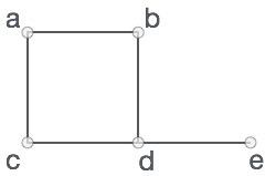

In the above graph,

V = {a, b, c, d, e}
E = {ab, ac, bd, cd, de}

Example

We can present this graph in a python program as below −

# Create the dictionary with graph elements
graph = { 
   "a" : ["b","c"],
   "b" : ["a", "d"],
   "c" : ["a", "d"],
   "d" : ["e"],
   "e" : ["d"]
}
# Print the graph 		 
print(graph)

Output

When the above code is executed, it produces the following result −

{'c': ['a', 'd'], 'a': ['b', 'c'], 'e': ['d'], 'd': ['e'], 'b': ['a', 'd']}

Display graph vertices

To display the graph vertices we simple find the keys of the graph dictionary. We use the keys() method.

class graph:
   def __init__(self,gdict=None):
      if gdict is None:
         gdict = []
      self.gdict = gdict
# Get the keys of the dictionary
   def getVertices(self):
      return list(self.gdict.keys())
# Create the dictionary with graph elements
graph_elements = { 
   "a" : ["b","c"],
   "b" : ["a", "d"],
   "c" : ["a", "d"],
   "d" : ["e"],
   "e" : ["d"]
}
g = graph(graph_elements)
print(g.getVertices())

Output

When the above code is executed, it produces the following result −

['d', 'b', 'e', 'c', 'a']

Display graph edges

Finding the graph edges is little tricker than the vertices as we have to find each of the pairs of vertices which have an edge in between them. So we create an empty list of edges then iterate through the edge values associated with each of the vertices. A list is formed containing the distinct group of edges found from the vertices.

class graph:
   def __init__(self,gdict=None):
      if gdict is None:
         gdict = {}
      self.gdict = gdict

   def edges(self):
      return self.findedges()
# Find the distinct list of edges
   def findedges(self):
      edgename = []
      for vrtx in self.gdict:
         for nxtvrtx in self.gdict[vrtx]:
            if {nxtvrtx, vrtx} not in edgename:
               edgename.append({vrtx, nxtvrtx})
      return edgename
# Create the dictionary with graph elements
graph_elements = { 
   "a" : ["b","c"],
   "b" : ["a", "d"],
   "c" : ["a", "d"],
   "d" : ["e"],
   "e" : ["d"]
}
g = graph(graph_elements)
print(g.edges())

Output

When the above code is executed, it produces the following result −

[{'b', 'a'}, {'b', 'd'}, {'e', 'd'}, {'a', 'c'}, {'c', 'd'}]

Adding a vertex

Adding a vertex is straight forward where we add another additional key to the graph dictionary.

Example

class graph:
   def __init__(self,gdict=None):
      if gdict is None:
         gdict = {}
      self.gdict = gdict
   def getVertices(self):
      return list(self.gdict.keys())
# Add the vertex as a key
   def addVertex(self, vrtx):
      if vrtx not in self.gdict:
         self.gdict[vrtx] = []
# Create the dictionary with graph elements
graph_elements = { 
   "a" : ["b","c"],
   "b" : ["a", "d"],
   "c" : ["a", "d"],
   "d" : ["e"],
   "e" : ["d"]
}
g = graph(graph_elements)
g.addVertex("f")
print(g.getVertices())

Output

When the above code is executed, it produces the following result −

['a', 'b', 'c', 'd', 'e','f']

Adding an edge

Adding an edge to an existing graph involves treating the new vertex as a tuple and validating if the edge is already present. If not then the edge is added.

class graph:
   def __init__(self,gdict=None):
      if gdict is None:
         gdict = {}
      self.gdict = gdict
   def edges(self):
      return self.findedges()
# Add the new edge
   def AddEdge(self, edge):
      edge = set(edge)
      (vrtx1, vrtx2) = tuple(edge)
      if vrtx1 in self.gdict:
         self.gdict[vrtx1].append(vrtx2)
      else:
         self.gdict[vrtx1] = [vrtx2]
# List the edge names
   def findedges(self):
      edgename = []
      for vrtx in self.gdict:
         for nxtvrtx in self.gdict[vrtx]:
            if {nxtvrtx, vrtx} not in edgename:
               edgename.append({vrtx, nxtvrtx})
        return edgename
# Create the dictionary with graph elements
graph_elements = { 
   "a" : ["b","c"],
   "b" : ["a", "d"],
   "c" : ["a", "d"],
   "d" : ["e"],
   "e" : ["d"]
}
g = graph(graph_elements)
g.AddEdge({'a','e'})
g.AddEdge({'a','c'})
print(g.edges())

Output

When the above code is executed, it produces the following result −

[{'e', 'd'}, {'b', 'a'}, {'b', 'd'}, {'a', 'c'}, {'a', 'e'}, {'c', 'd'}]

Python - Algorithm Design

Algorithm is a step-by-step procedure, which defines a set of instructions to be executed in a certain order to get the desired output. Algorithms are generally created independent of underlying languages, i.e. an algorithm can be implemented in more than one programming language.

From the data structure point of view, following are some important categories of algorithms −

• Search − Algorithm to search an item in a data structure.

• Sort − Algorithm to sort items in a certain order.

• Insert − Algorithm to insert item in a data structure.

• Update − Algorithm to update an existing item in a data structure.

• Delete − Algorithm to delete an existing item from a data structure.

Characteristics of an Algorithm

Not all procedures can be called an algorithm. An algorithm should have the following characteristics −

• Unambiguous − Algorithm should be clear and unambiguous. Each of its steps (or phases), and their inputs/outputs should be clear and must lead to only one meaning.

• Input − An algorithm should have 0 or more well-defined inputs.

• Output − An algorithm should have 1 or more well-defined outputs, and should match the desired output.

• Finiteness − Algorithms must terminate after a finite number of steps.

• Feasibility − Should be feasible with the available resources.

• Independent − An algorithm should have step-by-step directions, which should be independent of any programming code.

How to Write an Algorithm?

There are no well-defined standards for writing algorithms. Rather, it is problem and resource dependent. Algorithms are never written to support a particular programming code.

As we know that all programming languages share basic code constructs like loops (do, for, while), flow-control (if-else), etc. These common constructs can be used to write an algorithm.

We write algorithms in a step-by-step manner, but it is not always the case. Algorithm writing is a process and is executed after the problem domain is well-defined. That is, we should know the problem domain, for which we are designing a solution.

Example

Let's try to learn algorithm-writing by using an example.

• Problem − Design an algorithm to add two numbers and display the result.

step 1 − START

step 2 − declare three integers a, b & c

step 3 − define values of a & b

step 4 − add values of a & b

step 5 − store output of step 4 to c

step 6 − print c

step 7 − STOP

Algorithms tell the programmers how to code the program. Alternatively, the algorithm can be written as −

step 1 − START ADD

step 2 − get values of a & b

step 3 − c ← a + b

step 4 − display c

step 5 − STOP

In design and analysis of algorithms, usually the second method is used to describe an algorithm. It makes it easy for the analyst to analyze the algorithm ignoring all unwanted definitions. He can observe what operations are being used and how the process is flowing.

Writing step numbers, is optional.

We design an algorithm to get a solution of a given problem. A problem can be solved in more than one ways.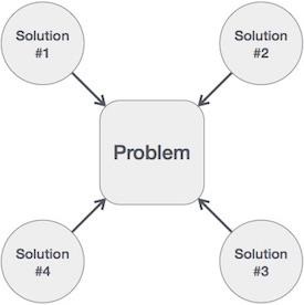

Hence, many solution algorithms can be derived for a given problem. The next step is to analyze those proposed solution algorithms and implement the best suitable solution.

Python - Divide and Conquer

In divide and conquer approach, the problem in hand, is divided into smaller sub-problems and then each problem is solved independently. When we keep on dividing the subproblems into even smaller sub-problems, we may eventually reach a stage where no more division is possible. Those "atomic" smallest possible sub-problem (fractions) are solved. The solution of all sub-problems is finally merged in order to obtain the solution of an original problem.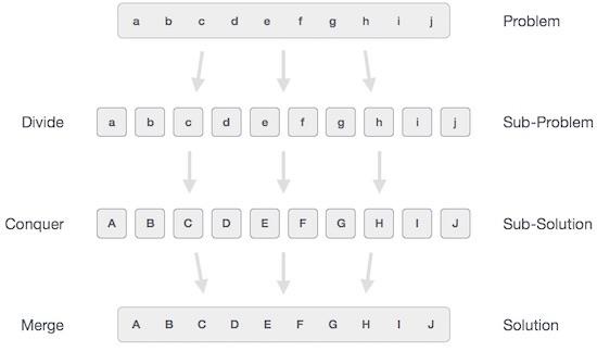

Broadly, we can understand divide-and-conquer approach in a three-step process.

Divide/Break

This step involves breaking the problem into smaller sub-problems. Sub-problems should represent a part of the original problem. This step generally takes a recursive approach to divide the problem until no sub-problem is further divisible. At this stage, sub-problems become atomic in nature but still represent some part of the actual problem.

Conquer/Solve

This step receives a lot of smaller sub-problems to be solved. Generally, at this level, the problems are considered 'solved' on their own.

Merge/Combine

When the smaller sub-problems are solved, this stage recursively combines them until they formulate a solution of the original problem. This algorithmic approach works recursively and conquer &amps; merge steps works so close that they appear as one.

Examples

The following program is an example of divide-and-conquer programming approach where the binary search is implemented using python.

Binary Search implementation

In binary search we take a sorted list of elements and start looking for an element at the middle of the list. If the search value matches with the middle value in the list we complete the search. Otherwise we eleminate half of the list of elements by choosing whether to procees with the right or left half of the list depending on the value of the item searched.

This is possible as the list is sorted and it is much quicker than linear search.Here we divide the given list and conquer by choosing the proper half of the list. We repeat this approcah till we find the element or conclude about it's absence in the list.

Example

def bsearch(list, val):
   list_size = len(list) - 1
   idx0 = 0
   idxn = list_size
# Find the middle most value
   while idx0 <= idxn:
      midval = (idx0 + idxn)// 2
      if list[midval] == val:
         return midval
# Compare the value the middle most value
   if val > list[midval]:
      idx0 = midval + 1
   else:
      idxn = midval - 1
   if idx0 > idxn:
      return None
# Initialize the sorted list
list = [2,7,19,34,53,72]

# Print the search result
print(bsearch(list,72))
print(bsearch(list,11))

Output

When the above code is executed, it produces the following result −

5
None

Python - Recursion

Recursion allows a function to call itself. Fixed steps of code get executed again and again for new values. We also have to set criteria for deciding when the recursive call ends. In the below example we see a recursive approach to the binary search. We take a sorted list and give its index range as input to the recursive function.

Binary Search using Recursion

We implement the algorithm of binary search using python as shown below. We use an ordered list of items and design a recursive function to take in the list along with starting and ending index as input. Then, the binary search function calls itself till find the searched item or concludes about its absence in the list.

Example

def bsearch(list, idx0, idxn, val):
   if (idxn < idx0):
      return None
   else:
      midval = idx0 + ((idxn - idx0) // 2)
# Compare the search item with middle most value
   if list[midval] > val:
      return bsearch(list, idx0, midval-1,val)
   else if list[midval] < val:
      return bsearch(list, midval+1, idxn, val)
   else:
      return midval
list = [8,11,24,56,88,131]
print(bsearch(list, 0, 5, 24))
print(bsearch(list, 0, 5, 51))

Output

When the above code is executed, it produces the following result −

2
None

Python - Backtracking

Backtracking is a form of recursion. But it involves choosing only option out of any possibilities. We begin by choosing an option and backtrack from it, if we reach a state where we conclude that this specific option does not give the required solution. We repeat these steps by going across each available option until we get the desired solution.

Below is an example of finding all possible order of arrangements of a given set of letters. When we choose a pair we apply backtracking to verify if that exact pair has already been created or not. If not already created, the pair is added to the answer list else it is ignored.

Example

def permute(list, s):
   if list == 1:
      return s
   else:
      return [ 
         y + x
         for y in permute(1, s)
         for x in permute(list - 1, s)
      ]
print(permute(1, ["a","b","c"]))
print(permute(2, ["a","b","c"]))

Output

When the above code is executed, it produces the following result −

['a', 'b', 'c']
['aa', 'ab', 'ac', 'ba', 'bb', 'bc', 'ca', 'cb', 'cc']

Python - Sorting Algorithms

Sorting refers to arranging data in a particular format. Sorting algorithm specifies the way to arrange data in a particular order. Most common orders are in numerical or lexicographical order.

The importance of sorting lies in the fact that data searching can be optimized to a very high level, if data is stored in a sorted manner. Sorting is also used to represent data in more readable formats. Below we see five such implementations of sorting in python.

• Bubble Sort

• Merge Sort

• Insertion Sort

• Shell Sort

• Selection Sort

Bubble Sort

It is a comparison-based algorithm in which each pair of adjacent elements is compared and the elements are swapped if they are not in order.

Example

def bubblesort(list):

# Swap the elements to arrange in order
   for iter_num in range(len(list)-1,0,-1):
      for idx in range(iter_num):
         if list[idx]>list[idx+1]:
            temp = list[idx]
            list[idx] = list[idx+1]
            list[idx+1] = temp
list = [19,2,31,45,6,11,121,27]
bubblesort(list)
print(list)

Output

When the above code is executed, it produces the following result −

[2, 6, 11, 19, 27, 31, 45, 121]

Merge Sort

Merge sort first divides the array into equal halves and then combines them in a sorted manner.

Example

def merge_sort(unsorted_list):
   if len(unsorted_list) <= 1:
      return unsorted_list
# Find the middle point and devide it
   middle = len(unsorted_list) // 2
   left_list = unsorted_list[:middle]
   right_list = unsorted_list[middle:]

   left_list = merge_sort(left_list)
   right_list = merge_sort(right_list)
   return list(merge(left_list, right_list))

# Merge the sorted halves
def merge(left_half,right_half):
   res = []
   while len(left_half) != 0 and len(right_half) != 0:
      if left_half[0] < right_half[0]:
         res.append(left_half[0])
         left_half.remove(left_half[0])
      else:
         res.append(right_half[0])
         right_half.remove(right_half[0])
   if len(left_half) == 0:
      res = res + right_half
   else:
      res = res + left_half
   return res
unsorted_list = [64, 34, 25, 12, 22, 11, 90]
print(merge_sort(unsorted_list))

Output

When the above code is executed, it produces the following result −

[11, 12, 22, 25, 34, 64, 90]

Insertion Sort

Insertion sort involves finding the right place for a given element in a sorted list. So in beginning we compare the first two elements and sort them by comparing them. Then we pick the third element and find its proper position among the previous two sorted elements. This way we gradually go on adding more elements to the already sorted list by putting them in their proper position.

Example

def insertion_sort(InputList):
   for i in range(1, len(InputList)):
      j = i-1
      nxt_element = InputList[i]
# Compare the current element with next one
   while (InputList[j] > nxt_element) and (j >= 0):
      InputList[j+1] = InputList[j]
      j=j-1
   InputList[j+1] = nxt_element
list = [19,2,31,45,30,11,121,27]
insertion_sort(list)
print(list)

Output

When the above code is executed, it produces the following result −

[19, 2, 31, 45, 30, 11, 27, 121]

Shell Sort

Shell Sort involves sorting elements which are away from each other. We sort a large sublist of a given list and go on reducing the size of the list until all elements are sorted. The below program finds the gap by equating it to half of the length of the list size and then starts sorting all elements in it. Then we keep resetting the gap until the entire list is sorted.

Example

def shellSort(input_list):
   gap = len(input_list) // 2
   while gap > 0:
      for i in range(gap, len(input_list)):
         temp = input_list[i]
         j = i
# Sort the sub list for this gap
   while j >= gap and input_list[j - gap] > temp:
      input_list[j] = input_list[j - gap]
      j = j-gap
      input_list[j] = temp
# Reduce the gap for the next element
   gap = gap//2
list = [19,2,31,45,30,11,121,27]
shellSort(list)
print(list)

Output

When the above code is executed, it produces the following result −

[2, 11, 19, 27, 30, 31, 45, 121]

Selection Sort

In selection sort we start by finding the minimum value in a given list and move it to a sorted list. Then we repeat the process for each of the remaining elements in the unsorted list. The next element entering the sorted list is compared with the existing elements and placed at its correct position.So, at the end all the elements from the unsorted list are sorted.

Example

def selection_sort(input_list):
   for idx in range(len(input_list)):
      min_idx = idx
      for j in range( idx +1, len(input_list)):
         if input_list[min_idx] > input_list[j]:
            min_idx = j
# Swap the minimum value with the compared value
   input_list[idx], input_list[min_idx] = input_list[min_idx], input_list[idx]
l = [19,2,31,45,30,11,121,27]
selection_sort(l)
print(l)

Output

When the above code is executed, it produces the following result −

[19, 2, 31, 45, 30, 11, 121, 27]

Python - Searching Algorithms

Searching is a very basic necessity when you store data in different data structures. The simplest approach is to go across every element in the data structure and match it with the value you are searching for.This is known as Linear search. It is inefficient and rarely used, but creating a program for it gives an idea about how we can implement some advanced search algorithms.

Linear Search

In this type of search, a sequential search is made over all items one by one. Every item is checked and if a match is found then that particular item is returned, otherwise the search continues till the end of the data structure.

Example

def linear_search(values, search_for):
   search_at = 0
   search_res = False
# Match the value with each data element	
   while search_at < len(values) and search_res is False:
      if values[search_at] == search_for:
         search_res = True
      else:
         search_at = search_at + 1
   return search_res
l = [64, 34, 25, 12, 22, 11, 90]
print(linear_search(l, 12))
print(linear_search(l, 91))

Output

When the above code is executed, it produces the following result −

True
False

Interpolation Search

This search algorithm works on the probing position of the required value. For this algorithm to work properly, the data collection should be in a sorted form and equally distributed.Initially, the probe position is the position of the middle most item of the collection.If a match occurs, then the index of the item is returned.If the middle item is greater than the item, then the probe position is again calculated in the sub-array to the right of the middle item. Otherwise, the item is searched in the subarray to the left of the middle item. This process continues on the sub-array as well until the size of subarray reduces to zero.

Example

There is a specific formula to calculate the middle position which is indicated in the program below −

def intpolsearch(values,x ):
   idx0 = 0
   idxn = (len(values) - 1)
   while idx0 <= idxn and x >= values[idx0] and x <= values[idxn]:
# Find the mid point
	mid = idx0 +\
      int(((float(idxn - idx0)/( values[idxn] - values[idx0]))
      * ( x - values[idx0])))
# Compare the value at mid point with search value 
   if values[mid] == x:
      return "Found "+str(x)+" at index "+str(mid)
   if values[mid] < x:
      idx0 = mid + 1
   return "Searched element not in the list"

l = [2, 6, 11, 19, 27, 31, 45, 121]
print(intpolsearch(l, 2))

Output

When the above code is executed, it produces the following result −

Found 2 at index 0

Python - Graph Algorithms

Graphs are very useful data structures in solving many important mathematical challenges. For example computer network topology or analysing molecular structures of chemical compounds. They are also used in city traffic or route planning and even in human languages and their grammar. All these applications have a common challenge of traversing the graph using their edges and ensuring that all nodes of the graphs are visited. There are two common established methods to do this traversal which is described below.

Depth First Traversal

Also called depth first search (DFS),this algorithm traverses a graph in a depth ward motion and uses a stack to remember to get the next vertex to start a search, when a dead end occurs in any iteration. We implement DFS for a graph in python using the set data types as they provide the required functionalities to keep track of visited and unvisited nodes.

Example

class graph:
   def __init__(self,gdict=None):
      if gdict is None:
         gdict = {}
      self.gdict = gdict
# Check for the visisted and unvisited nodes
def dfs(graph, start, visited = None):
   if visited is None:
      visited = set()
   visited.add(start)
   print(start)
   for next in graph[start] - visited:
      dfs(graph, next, visited)
   return visited

gdict = { 
   "a" : set(["b","c"]),
   "b" : set(["a", "d"]),
   "c" : set(["a", "d"]),
   "d" : set(["e"]),
   "e" : set(["a"])
}
dfs(gdict, 'a')

Output

When the above code is executed, it produces the following result −

a 
b 
d 
e 
c

Breadth First Traversal

Also called breadth first search (BFS),this algorithm traverses a graph breadth ward motion and uses a queue to remember to get the next vertex to start a search, when a dead end occurs in any iteration. Please visit this link in our website to understand the details of BFS steps for a graph.

We implement BFS for a graph in python using queue data structure discussed earlier. When we keep visiting the adjacent unvisited nodes and keep adding it to the queue. Then we start dequeue only the node which is left with no unvisited nodes. We stop the program when there is no next adjacent node to be visited.

Example

import collections
class graph:
   def __init__(self,gdict=None):
      if gdict is None:
         gdict = {}
      self.gdict = gdict
def bfs(graph, startnode):
# Track the visited and unvisited nodes using queue
   seen, queue = set([startnode]), collections.deque([startnode])
   while queue:
      vertex = queue.popleft()
      marked(vertex)
      for node in graph[vertex]:
         if node not in seen:
            seen.add(node)
            queue.append(node)

def marked(n):
   print(n)

# The graph dictionary
gdict = { 
   "a" : set(["b","c"]),
   "b" : set(["a", "d"]),
   "c" : set(["a", "d"]),
   "d" : set(["e"]),
   "e" : set(["a"])
}
bfs(gdict, "a")

Output

When the above code is executed, it produces the following result −

a 
c 
b 
d 
e 

Python - Algorithm Analysis

Efficiency of an algorithm can be analyzed at two different stages, before implementation and after implementation. They are the following −

• A Priori Analysis − This is a theoretical analysis of an algorithm. Efficiency of an algorithm is measured by assuming that all other factors, for example, processor speed, are constant and have no effect on the implementation.

• A Posterior Analysis − This is an empirical analysis of an algorithm. The selected algorithm is implemented using programming language. This is then executed on target computer machine. In this analysis, actual statistics like running time and space required, are collected.

Algorithm Complexity

Suppose X is an algorithm and n is the size of input data, the time and space used by the algorithm X are the two main factors, which decide the efficiency of X.

• Time Factor − Time is measured by counting the number of key operations such as comparisons in the sorting algorithm.

• Space Factor − Space is measured by counting the maximum memory space required by the algorithm.

The complexity of an algorithm f(n) gives the running time and/or the storage space required by the algorithm in terms of n as the size of input data.

Space Complexity

Space complexity of an algorithm represents the amount of memory space required by the algorithm in its life cycle. The space required by an algorithm is equal to the sum of the following two components −

• A fixed part that is a space required to store certain data and variables, that are independent of the size of the problem. For example, simple variables and constants used, program size, etc.

• A variable part is a space required by variables, whose size depends on the size of the problem. For example, dynamic memory allocation, recursion stack space, etc.

Space complexity S(P) of any algorithm P is S(P) = C + SP(I), where C is the fixed part and S(I) is the variable part of the algorithm, which depends on instance characteristic I. Following is a simple example that tries to explain the concept −

Algorithm: SUM(A, B)

Step 1 − START

Step 2 − C ← A + B + 10

Step 3 − Stop

Here we have three variables A, B, and C and one constant. Hence S(P) = 1 + 3. Now, space depends on data types of given variables and constant types and it will be multiplied accordingly.

Time Complexity

Time complexity of an algorithm represents the amount of time required by the algorithm to run to completion. Time requirements can be defined as a numerical function T(n), where T(n) can be measured as the number of steps, provided each step consumes constant time.

For example, addition of two n-bit integers takes n steps. Consequently, the total computational time is T(n) = c ∗ n, where c is the time taken for the addition of two bits. Here, we observe that T(n) grows linearly as the input size increases.

Python - Algorithm Types

The efficiency and accuracy of algorithms have to be analysed to compare them and choose a specific algorithm for certain scenarios. The process of making this analysis is called Asymptotic analysis. It refers to computing the running time of any operation in mathematical units of computation.

For example, the running time of one operation is computed as f(n) and may be for another operation it is computed as g(n2). This means the first operation running time will increase linearly with the increase in n and the running time of the second operation will increase exponentially when n increases. Similarly, the running time of both operations will be nearly the same if n is significantly small.

Usually, the time required by an algorithm falls under three types −

• Best Case − Minimum time required for program execution.

• Average Case − Average time required for program execution.

• Worst Case − Maximum time required for program execution.

Asymptotic Notations

The commonly used asymptotic notations to calculate the running time complexity of an algorithm.

• Ο Notation

• Ω Notation

• θ Notation

Big Oh Notation, Ο

The notation Ο(n) is the formal way to express the upper bound of an algorithm's running time. It measures the worst case time complexity or the longest amount of time an algorithm can possibly take to complete.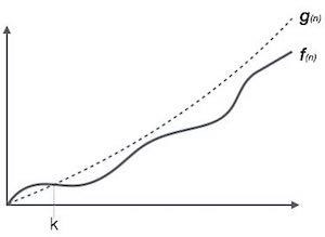

For example, for a function f(n)

Ο(f(n)) = { g(n) : there exists c > 0 and n0 such that f(n) ≤ c.g(n) for all n > n0. }

Omega Notation, Ω

The notation Ω(n) is the formal way to express the lower bound of an algorithm's running time. It measures the best case time complexity or the best amount of time an algorithm can possibly take to complete.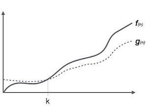

For example, for a function f(n)

Ω(f(n)) ≥ { g(n) : there exists c > 0 and n0 such that g(n) ≤ c.f(n) for all n > n0. }

Theta Notation, θ

The notation θ(n) is the formal way to express both the lower bound and the upper bound of an algorithm's running time. It is represented as follows −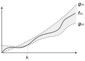

θ(f(n)) = { g(n) if and only if g(n) =  Ο(f(n)) and g(n) = Ω(f(n)) for all n > n0. }

Common Asymptotic Notations

A list of some common asymptotic notations is mentioned below −

Python - Algorithm Classes

Algorithms are unambiguous steps which should give us a well-defined output by processing zero or more inputs. This leads to many approaches in designing and writing the algorithms. It has been observed that most of the algorithms can be classified into the following categories.

Greedy Algorithms

Greedy algorithms try to find a localized optimum solution, which may eventually lead to globally optimized solutions. However, generally greedy algorithms do not provide globally optimized solutions.

So greedy algorithms look for a easy solution at that point in time without considering how it impacts the future steps. It is similar to how humans solve problems without going through the complete details of the inputs provided.

Most networking algorithms use the greedy approach. Here is a list of few of them −

• Travelling Salesman Problem

• Prim's Minimal Spanning Tree Algorithm

• Kruskal's Minimal Spanning Tree Algorithm

• Dijkstra's Minimal Spanning Tree Algorithm

Divide and Conquer

This class of algorithms involve dividing the given problem into smaller sub-problems and then solving each of the sub-problem independently. When the problem can not be further sub divided, we start merging the solution to each of the sub-problem to arrive at the solution for the bigger problem.

The important examples of divide and conquer algorithms are −

• Merge Sort

• Quick Sort

• Kruskal's Minimal Spanning Tree Algorithm

• Binary Search

Dynamic Programming

Dynamic programming involves dividing the bigger problem into smaller ones but unlike divide and conquer it does not involve solving each sub-problem independently. Rather the results of smaller sub-problems are remembered and used for similar or overlapping sub-problems.

Mostly, these algorithms are used for optimization. Before solving the in-hand sub-problem, dynamic algorithm will try to examine the results of the previously solved sub-problems.Dynamic algorithms are motivated for an overall optimization of the problem and not the local optimization.

The important examples of Dynamic programming algorithms are −

• Fibonacci number series

• Knapsack problem

• Tower of Hanoi

Python - Amortized Analysis

Amortized analysis involves estimating the run time for the sequence of operations in a program without taking into consideration the span of the data distribution in the input values. A simple example is finding a value in a sorted list is quicker than in an unsorted list.

If the list is already sorted, it does not matter how distributed the data is. But of course the length of the list has an impact as it decides the number of steps the algorithm has to go through to get the final result.

So we see that if the initial cost of a single step of obtaining a sorted list is high, then the cost of subsequent steps of finding an element becomes considerably low. So Amortized analysis helps us find a bound on the worst-case running time for a sequence of operations. There are three approaches to amortized analysis.

• Accounting Method − This involves assigning a cost to each operation performed. If the actual operation finishes quicker than the assigned time then some positive credit is accumulated in the analysis.

In the reverse scenario it will be negative credit. To keep track of these accumulated credits, we use a stack or tree data structure. The operations which are carried out early ( like sorting the list) have high amortized cost but the operations that are late in sequence have lower amortized cost as the accumulated credit is utilized. So the amortized cost is an upper bound of actual cost.

• Potential Method − In this method the saved credit is utilized for future operations as mathematical function of the state of the data structure. The evaluation of the mathematical function and the amortized cost should be equal. So when the actual cost is greater than amortized cost there is a decrease in potential and it is used utilized for future operations which are expensive.

• Aggregate analysis − In this method we estimate the upper bound on the total cost of n steps. The amortized cost is a simple division of total cost and the number of steps (n)..

Python - Algorithm Justifications

In order to make claims about an Algorithm being efficient we need some mathematical tools as proof. These tools help us on providing a mathematically satisfying explanation on the performance and accuracy of the algorithms. Below is a list of some of those mathematical tools which can be used for justifying one algorithm over another.

• Direct Proof − It is direct verification of the statement by using the direct calculations. For example sum of two even numbers is always an even number. In this case just add the two numbers you are investigating and verify the result as even.

• Proof by induction − Here we start with a specific instance of a truth and then generalize it to all possible values which are part of the truth. The approach is to take a case of verified truth, then prove it is also true for the next case for the same given condition. For example all positive numbers of the form 2n-1 are odd. We prove it for a certain value of n, then prove it for the next value of n. This establishes the statement as generally true by proof of induction.

• Proof by contraposition − This proof is based on the condition If Not A implies Not B then A implies B. A simple example is if square of n is even then n must be even. Because if square on n is not even then n is not even.

• Proof by exhaustion − This is similar to direct proof but it is established by visiting each case separately and proving each of them. An example of such proof is the four color theorem.