Chapter 18Duality

In this chapter, we review duality principles in optimization.

18.1 Dual norms

We introduce in this section dual norms, since they are useful in this book.

Definition 18.1 (Dual norms)

Given a norm $∥ u ∥$ ∥u∥, its dual is $∥ v ∥_{*} ≔ \max_{∥ u ∥ \leq 1} ⟨ u, v ⟩ .$ ∥v∥∗:=∥u∥≤1max⟨u,v⟩.

Therefore, the dual norm of $∥ \cdot ∥$ ∥⋅∥ is the support function of the unit ball induced by the norm $∥ \cdot ∥$ ∥⋅∥, $B_{∥ \cdot ∥} ≔ {u \in R^{D} ⁣ : ∥ u ∥ \leq 1} .$ B∥⋅∥:={u∈RD:∥u∥≤1}. We give examples of pairs of dual norms below.

Example 18.1 (Dual norm of $p$ p-norms)

The $p$ p-norm is defined by $∥ u ∥_{p} ≔ {(\sum_{j = 1}^{D} ∣ u_{j} ∣^{p})}^{1 / p} .$ ∥u∥p:=(j=1∑D∣uj∣p)1/p. Its dual is $∥ v ∥_{q}$ ∥v∥q where $q$ q is such that $\frac{1}{p} + \frac{1}{q} = 1$ p1+q1=1. For instance, the dual norm of the $2$ 2-norm is itself, since $\frac{1}{2} + \frac{1}{2} = 1$ 21+21=1. The $1$ 1-norm and the $\infty$ ∞-norm are duals of each other, since $\frac{1}{1} + \frac{1}{\infty} = 1$ 11+∞1=1.

The definition of dual norm implies a generalization of the Cauchy–Schwarz inequality: for all $u, v \in R^{D}$ u,v∈RD $∣ ⟨ u, v ⟩ ∣ \leq ∥ u ∥_{*} ∥ v ∥ .$ ∣⟨u,v⟩∣≤∥u∥∗∥v∥. See, e.g., Beck (2017, Lemma 1.4).

Proposition 18.1 (Conjugate of norms and squared norms)

We know that the conjugate of the support function is the indicator function. Therefore, if $f (u) = ∥ u ∥$ f(u)=∥u∥, then $f^{*} (v) = ι_{B_{∥ \cdot ∥}} (v) = {\begin{matrix} 0 & if ∥ v ∥_{*} \leq 1 \\ \infty & otherwise \end{matrix} .$ f∗(v)=ιB∥⋅∥(v)={0∞ if ∥v∥∗≤1 otherwise . On the other hand, if $f (u) = \frac{1}{2} ∥ u ∥^{2}$ f(u)=21∥u∥2, then $f^{*} (v) = \frac{1}{2} ∥ v ∥_{*}^{2} .$ f∗(v)=21∥v∥∗2.

18.2 Fenchel duality

We consider in this section standard objectives of the form $\min_{w \in W} L (w) ≔ \min_{w \in W} ℓ (f (w)) + R (w),$ w∈WminL(w):=w∈Wminℓ(f(w))+R(w), where $f ⁣ : W \to M$ f:W→M, $ℓ ⁣ : M \to R$ ℓ:M→R and $R ⁣ : W \to R$ R:W→R. We first show that the minimization of this objective, called the primal, can be lower bounded by a concave maximization objective, called the dual, even if the primal is nonconvex.

Proposition 18.2 (Weak duality)

Let $f ⁣ : W \to M$ f:W→M (potentially nonlinear), $ℓ ⁣ : M \to R$ ℓ:M→R (potentially nonconvex) and $R ⁣ : W \to R$ R:W→R (potentially nonconvex). Then $\min_{w \in W} ℓ (f (w)) + R (w) \geq \max_{α \in M} - R^{f} (α) - ℓ^{*} (- α),$ w∈Wminℓ(f(w))+R(w)≥α∈Mmax−Rf(α)−ℓ∗(−α), where we used the conjugate $ℓ^{*} (- α) ≔ \max_{θ \in M} ⟨ - α, θ ⟩ - ℓ (θ)$ ℓ∗(−α):=θ∈Mmax⟨−α,θ⟩−ℓ(θ) and the “generalized conjugate” $R^{f} (α) ≔ \max_{w \in W} ⟨ α, f (w) ⟩ - R (w) .$ Rf(α):=w∈Wmax⟨α,f(w)⟩−R(w). Moreover, $ℓ^{*}$ ℓ∗ and $R^{f}$ Rf are both convex functions.

We emphasize that the result in Proposition 18.2 is fully general, in the sense that it does not assume the linearity of $f$ f or the convexity of $ℓ$ ℓ and $R$ R. The caveat, of course, is that $R^{f}$ Rf and $ℓ^{*}$ ℓ∗ are difficult to compute in general, if $f$ f is nonlinear, and if $ℓ$ ℓ and $R$ R are nonconvex.

Proof

$\begin{matrix} \min_{w \in W} ℓ (f (w)) + R (w) \\ = & \min_{\begin{matrix} w \in W \\ θ \in M \end{matrix}} ℓ (θ) + R (w) s.t. θ = f (w) \\ = & \min_{\begin{matrix} w \in W \\ θ \in M \end{matrix}} \max_{α \in M} ℓ (θ) + R (w) + ⟨ α, θ - f (w) ⟩ \\ \geq & \max_{α \in M} \min_{\begin{matrix} w \in W \\ θ \in M \end{matrix}} ℓ (θ) + R (w) + ⟨ α, θ - f (w) ⟩ \\ = & \max_{α \in M} \min_{w \in W} ⟨ α, - f (w) ⟩ + R (w) + \min_{θ \in M} ℓ (θ) + ⟨ α, θ ⟩ \\ = & \max_{α \in M} - \max_{w \in W} ⟨ α, f (w) ⟩ - R (w) - \max_{θ \in M} ⟨ - α, θ ⟩ - ℓ (θ) \\ = & \max_{α \in M} - R^{f} (α) - ℓ^{*} (- α) . \end{matrix}$ ==≥===w∈Wminℓ(f(w))+R(w)w∈Wθ∈Mminℓ(θ)+R(w)s.t.θ=f(w)w∈Wθ∈Mminα∈Mmaxℓ(θ)+R(w)+⟨α,θ−f(w)⟩α∈Mmaxw∈Wθ∈Mminℓ(θ)+R(w)+⟨α,θ−f(w)⟩α∈Mmaxw∈Wmin⟨α,−f(w)⟩+R(w)+θ∈Mminℓ(θ)+⟨α,θ⟩α∈Mmax−w∈Wmax⟨α,f(w)⟩−R(w)−θ∈Mmax⟨−α,θ⟩−ℓ(θ)α∈Mmax−Rf(α)−ℓ∗(−α). ◻

In the case when $f (w) = A w$ f(w)=Aw, where $A$ A is a linear map, and when both $ℓ$ ℓ and $R$ R are convex, we can state a much stronger result.

Proposition 18.3 (Strong duality)

Let $A$ A be a linear map from $W$ W to $M$ M. Let $ℓ ⁣ : M \to R$ ℓ:M→R and $R ⁣ : W \to R$ R:W→R be convex functions. Let $A^{*}$ A∗ denote the adjoint of $A$ A (Section 2.3). Then, $\min_{w \in W} ℓ (A w) + R (w) = \max_{α \in M} - R^{*} (A^{*} α) - ℓ^{*} (- α) .$ w∈Wminℓ(Aw)+R(w)=α∈Mmax−R∗(A∗α)−ℓ∗(−α). Furthermore, the primal solution satisfies $w^{⋆} \in \underset{w \in W}{arg max} ⟨ A α^{⋆}, w ⟩ - R (w) .$ w⋆∈w∈Wargmax⟨Aα⋆,w⟩−R(w). When $R$ R is strictly convex, the primal solution is uniquely determined by $w^{⋆} = \nabla R^{*} (A^{*} α^{⋆}) .$ w⋆=∇R∗(A∗α⋆).

Proof

Since $f (w) = A w$ f(w)=Aw, we have $\begin{matrix} R^{f} (α) & ≔ \max_{w \in W} ⟨ α, f (w) ⟩ - R (w) \\ = \max_{w \in W} ⟨ α, A w ⟩ - R (w) \\ = \max_{w \in W} ⟨ A^{*} α, w ⟩ - R (w) \\ = R^{*} (A^{*} α) . \end{matrix}$ Rf(α):=w∈Wmax⟨α,f(w)⟩−R(w)=w∈Wmax⟨α,Aw⟩−R(w)=w∈Wmax⟨A∗α,w⟩−R(w)=R∗(A∗α). Furthermore, the inequality in the proof of Proposition 18.2 is an equality, since the $\min \max$ minmax is that of a convex-concave function. ◻

The maximization problem in Proposition 18.3 is called the Fenchel dual. By strong duality, the value of the maximum and the value of the minimum are equal. We can therefore choose to equivalently solve the dual instead of the primal. This can be advantageous when the space $M$ M is smaller than $W$ W.

We now apply the Fenchel dual to obtain the dual of regularized multiclass linear classification.

Example 18.2 (Sum of separable loss functions)

When the loss is
$ℓ (θ) ≔ \sum_{i = 1}^{N} ℓ_{i} (θ_{i})$ ℓ(θ):=∑i=1Nℓi(θi), where $θ = A w = (A_{1} w, \dots, A_{N} w) \in M^{N}$ θ=Aw=(A1w,…,ANw)∈MN and $A_{i}$ Ai is a linear map from $W$ W to $M$ M, we obtain $\min_{w \in W} \sum_{i = 1}^{N} ℓ_{i} (A_{i} w) + R (w) = \max_{α \in M^{N}} - R^{*} (A^{*} α) - \sum_{i = 1}^{N} ℓ_{i}^{*} (- α_{i}),$ w∈Wmini=1∑Nℓi(Aiw)+R(w)=α∈MNmax−R∗(A∗α)−i=1∑Nℓi∗(−αi), where $A^{*} α = (A_{1}^{*} α_{1}, \dots, A_{N}^{*} α_{N})$ A∗α=(A1∗α1,…,AN∗αN). Typically, we define $A_{i} w ≔ W x_{i},$ Aiw:=Wxi, where $W \in R^{M \times D}$ W∈RM×D is a reshaped version of $w \in W$ w∈W, $x_{i} \in R^{D}$ xi∈RD is a training sample, and $M$ M is the number of classes. In this case, we then have $A_{i}^{*} α_{i} = α_{i} x_{i}^{⊤} .$ Ai∗αi=αixi⊤.

Examples of loss function conjugates are given in Table 18.1.

Table 18.1: Examples of loss conjugates. For regression losses (squared, absolute), where $y_{i} \in R^{M}$ yi∈RM, we define $t_{i} = ϕ (y_{i}) = y_{i}$ ti=ϕ(yi)=yi. For classification losses (logistic, perceptron, hinge), where $y_{i} \in [M]$ yi∈[M], we define $t_{i} = ϕ (y_{i}) = e_{y_{i}}$ ti=ϕ(yi)=eyi. To simplify some expressions, we defined the change of variable $μ_{i} ≔ y_{i} - α_{i}$ μi:=yi−αi.

	$ℓ_{i} (θ_{i})$ ℓi(θi)	$ℓ_{i}^{*} (- α_{i})$ ℓi∗(−αi)
Squared	$\frac{1}{2} ∥ θ_{i} - t_{i} ∥_{2}^{2}$ 21∥θi−ti∥22	$\frac{1}{2} ∥ α_{i} ∥_{2}^{2} - ⟨ t_{i}, α_{i} ⟩$ 21∥αi∥22−⟨ti,αi⟩
Absolute	$∥ θ_{i} - t_{i} ∥_{1}$ ∥θi−ti∥1	$ι_{[- 1, 1]^{M}} (α_{i}) - ⟨ t_{i}, α_{i} ⟩$ ι[−1,1]M(αi)−⟨ti,αi⟩
Logistic	$L S E (θ_{i}) - ⟨ θ_{i}, t_{i} ⟩$ LSE(θi)−⟨θi,ti⟩	$⟨ μ_{i}, \log μ_{i} ⟩ + ι_{△^{M}} (μ_{i})$ ⟨μi,logμi⟩+ι△M(μi)
Perceptron	$\max_{j \in [M]} θ_{i, j} - θ_{i, y_{i}}$ maxj∈[M]θi,j−θi,yi	$ι_{△^{M}} (μ_{i})$ ι△M(μi)
Hinge	$\max_{j \in [M]} [j \neq y_{i}] + θ_{i, j} - θ_{i, y_{i}}$ maxj∈[M][j=yi]+θi,j−θi,yi	$ι_{△^{M}} (μ_{i}) - ⟨ 1 - t_{i}, μ_{i} ⟩$ ι△M(μi)−⟨1−ti,μi⟩

18.3 Bregman divergences

Bregman divergences are a measure of difference between two points.

Definition 18.2 (Bregman divergence)

The Bregman divergence generated by a differentiable convex function $f ⁣ : R^{D} \to R$ f:RD→R is $\begin{matrix} B_{f} (u, v) & ≔ f (u) - f (v) - ⟨ \nabla f (v), u - v ⟩ \\ = ⟨ \nabla f (v), v ⟩ - f (v) - [⟨ \nabla f (v), u ⟩ - f (u)], \end{matrix}$ Bf(u,v):=f(u)−f(v)−⟨∇f(v),u−v⟩=⟨∇f(v),v⟩−f(v)−[⟨∇f(v),u⟩−f(u)], where $u, v \in dom (f)$ u,v∈dom(f).

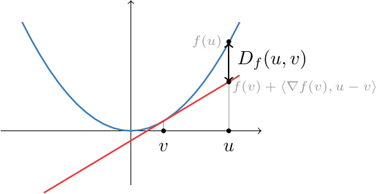
Intuitively, the Bregman divergence is the difference between $f (u)$ f(u) and its linearization $u \mapsto f (v) + ⟨ \nabla f (v), u - v ⟩$ u↦f(v)+⟨∇f(v),u−v⟩ around $v$ v. This is illustrated in Fig. 18.1.

Example 18.3 (Examples of Bregman divergences)

If $f (u) = \frac{1}{2} ∥ u ∥_{2}^{2}$ f(u)=21∥u∥22, where $dom (f) = R^{D}$ dom(f)=RD, then $B_{f} (u, v) = \frac{1}{2} ∥ u - v ∥_{2}^{2},$ Bf(u,v)=21∥u−v∥22, the squared Euclidean distance. If $f (u) = ⟨ u, \log u ⟩$ f(u)=⟨u,logu⟩, where $dom (f) = R_{+}^{D}$ dom(f)=R+D, then $B_{f} (u, v) = \sum_{j = 1}^{D} u_{j} \log \frac{u_{j}}{v_{j}} - \sum_{j = 1}^{D} u_{j} + \sum_{j = 1}^{D} v_{j},$ Bf(u,v)=j=1∑Dujlogvjuj−j=1∑Duj+j=1∑Dvj, the (generalized) Kullback-Leibler divergence.

Properties

Bregman divergences enjoy several useful properties.

Proposition 18.4 (Properties of Bregman divergences)

Let $f ⁣ : R^{D} \to R$ f:RD→R be a differentiable convex function.

Non-negativity: $B_{f} (u, v) \geq 0$ Bf(u,v)≥0 for all $u, v \in dom (f)$ u,v∈dom(f).
Positivity: $B_{f} (u, v) = 0$ Bf(u,v)=0 if and only if $u = v$ u=v (when $f$ f is strictly convex).
Convexity: $B_{f} (u, v)$ Bf(u,v) is convex in $u$ u.
Dual-space form: $B_{f} (u, v) = B_{f^{*}} (b, a)$ Bf(u,v)=Bf∗(b,a), where $b = \nabla f (v) \in dom (f^{*})$ b=∇f(v)∈dom(f∗) and $a = \nabla f (u) \in dom (f^{*})$ a=∇f(u)∈dom(f∗).

Proof

The properties follow immediately from the convexity of $f (u)$ f(u).

From Definition 15.6.
From the uniqueness of minimizers.
From the fact that $u \mapsto B_{f} (u, v)$ u↦Bf(u,v) is the sum of $f (u)$ f(u) and a linear function of $u$ u.

◻

Figure 18.1: The Bregman divergence generated by $f$ f is the difference between $f (u)$ f(u) and its linearization around $v$ v.

The Bregman divergence can be used to define natural generalizations of the Euclidean projection and proximal operators, reviewed in Section 16.3 and Section 16.4.

Definition 18.3 (Bregman proximal and projection operators)

Let $v \in dom (f)$ v∈dom(f). The Bregman proximal operator is ${b p r o x}_{f, g} (v) ≔ \underset{u \in dom (f) \cap dom (g)}{arg min} B_{f} (u, v) + g (u) .$ bproxf,g(v):=u∈dom(f)∩dom(g)argminBf(u,v)+g(u). In particular, the Bregman projection onto $C \subseteq dom (f)$ C⊆dom(f) is ${b p r o j}_{f, C} (v) ≔ \underset{u \in C}{arg min} B_{f} (u, v) .$ bprojf,C(v):=u∈CargminBf(u,v).

It turns out that these operators are intimately connected to the gradient mapping of the convex conjugate.

Proposition 18.5 (Link with conjugate’s gradient)

If $Ω = f + g$ Ω=f+g, then for all $θ \in dom (f^{*})$ θ∈dom(f∗) $\nabla Ω^{*} (θ) = {b p r o x}_{f, g} (\nabla f^{*} (θ)) .$ ∇Ω∗(θ)=bproxf,g(∇f∗(θ)). In particular, if $Ω = f + ι_{C}$ Ω=f+ιC, then for all $θ \in dom (f^{*})$ θ∈dom(f∗) $\nabla Ω^{*} (θ) = {b p r o j}_{f, C} (\nabla f^{*} (θ)) .$ ∇Ω∗(θ)=bprojf,C(∇f∗(θ)).

We give two examples below.

Example 18.4 (Bregman projections on the simplex)

If $f (u) = \frac{1}{2} ∥ u ∥_{2}^{2}$ f(u)=21∥u∥22, then $\begin{matrix} {b p r o j}_{f, △^{D}} (v) = \underset{u \in △^{D}}{arg min} \frac{1}{2} ∥ u - v ∥_{2}^{2} . \end{matrix}$ bprojf,△D(v)=u∈△Dargmin21∥u−v∥22. If $f (u) = ⟨ u, \log u - 1 ⟩$ f(u)=⟨u,logu−1⟩, then $\begin{matrix} {b p r o j}_{f, △^{D}} (v) = \underset{u \in △^{D}}{arg min} K L (u, v) = s o f t a r g m a x (θ), \end{matrix}$ bprojf,△D(v)=u∈△DargminKL(u,v)=softargmax(θ), where $v = \nabla f^{*} (θ) = \exp (θ)$ v=∇f∗(θ)=exp(θ).

Therefore, the softmax can be seen as a projection onto the probability simplex in the Kullback-Leibler divergence sense!

18.4 Fenchel-Young loss functions

We end this chapter with a brief review of the Fenchel-Young family of loss functions (Blondel et al., 2020), which includes all loss functions in Table 18.1.

Definition 18.4 (Fenchel-Young loss)

The Fenchel-Young loss function generated by $Ω$ Ω is $ℓ_{Ω} (θ, t) ≔ Ω^{*} (θ) + Ω (t) - ⟨ θ, t ⟩$ ℓΩ(θ,t):=Ω∗(θ)+Ω(t)−⟨θ,t⟩ where $θ \in dom (Ω^{*})$ θ∈dom(Ω∗) and $t \in dom (Ω)$ t∈dom(Ω).

Typically, we set $θ = f (x, w)$ θ=f(x,w), where $f$ f is a model prediction function with parameters $w$ w and $t = ϕ (y)$ t=ϕ(y), where $ϕ ⁣ : Y \to dom (Ω)$ ϕ:Y→dom(Ω). For instance, suppose we work with categorical outputs $y \in [M]$ y∈[M]. Then, we can set $ϕ (y) = e_{y}$ ϕ(y)=ey, where $e_{y}$ ey is the one-hot encoding of $y$ y.

The important point to notice is that the Fenchel-Young loss is defined over arguments in mixed spaces: $θ$ θ belongs to the dual space, while $t$ t belongs to the primal space. In fact, the Fenchel-Young loss is intimately connected to the Bregman divergence, since $B_{Ω} (t, v) = Ω^{*} (θ) + Ω (t) - ⟨ θ, t ⟩$ BΩ(t,v)=Ω∗(θ)+Ω(t)−⟨θ,t⟩, if we set $θ = \nabla Ω (v)$ θ=∇Ω(v). The key properties of Fenchel-Young loss functions are summarized below.

Proposition 18.6 (Properties of Fenchel-Young loss functions)

Non-negativity: $ℓ_{Ω} (θ, t) \geq 0$ ℓΩ(θ,t)≥0 for all $θ \in dom (Ω^{*})$ θ∈dom(Ω∗) and $t \in dom (Ω)$ t∈dom(Ω).
Positivity: $ℓ_{Ω} (θ, t) = 0$ ℓΩ(θ,t)=0 if and only if $\nabla Ω^{*} (θ) = t$ ∇Ω∗(θ)=t, assuming $Ω$ Ω is strictly convex.
Convexity: $ℓ_{Ω} (θ, t)$ ℓΩ(θ,t) is convex in $θ$ θ (regardless of $Ω$ Ω) and in $t$ t (if $Ω$ Ω is convex).
Relation with composite Bregman divergence: $0 \leq \underset{possibly nonconvex in θ}{\underset{⏟}{B_{Ω} (t, \nabla Ω^{*} (θ))}} \leq \underset{convex in θ}{\underset{⏟}{ℓ_{Ω} (θ, t)}} .$ 0≤possibly nonconvex in θBΩ(t,∇Ω∗(θ))≤convex in θℓΩ(θ,t).

See Blondel et al. (2020) for an in-depth study of more properties.

18.5 Summary

The convex conjugate serves as a powerful abstraction in Fenchel duality, decoupling the dual expression and function-specific terms.
The convex conjugate is also tightly connected to Bregman divergences and can be used to derive the family of Fenchel-Young loss functions, which can be seen as primal-dual Bregman divergences.

GeezerVison

Chapter 18Duality

18.1 Dual norms

18.2 Fenchel duality

18.3 Bregman divergences

Properties

18.4 Fenchel-Young loss functions

18.5 Summary